Summary Of Adapter Based Performance Efficient Fine Tuning (PEFT) Techniques For Large Language Models

The two most common transfer learning techniques in NLP were feature-based transfer (generating input text embedding from a pre-trained large model and using it as a feature in your custom model) and fine-tuning (fine tuning the pre-trained model on custom data set). It is notoriously hard to fine tune Large Language Models (LLMs) for a specific task on custom domain specific dataset. Given their enormous size (e.g. GPT3 175B parameters , Google T5 Flan XXL [1] 11B parameters, Meta Llama[2] 65 billion parameters) ones needs mammoth computing horsepower and extremely large scale datasets to fine tune them on a specific task. Apart from the mentioned challenges, fine tuning LLMs on specific task may lead them to “forget” previously learnt information, a phenomena known as catastrophic forgetting.

In this blog I will provide high level overview of different Adapter[4] based parameter efficient fine tuning techniques used to fine tune LLMs. PEFT based methods make fine-tuning large language models feasible on consumer grade hardware using reasonably small datasets, e.g. Alpaca[3] used 52 k data points to fine tune Llama 7B parameter model on multiple tasks in ~3 hours using a Nvidia A100 GPU[5].

HuggingFace PEFT module has 4 types of performance efficient fine-tuning methods available under peft.PEFT_TYPE_TO_CONFIG_MAPPING

{
'PROMPT_TUNING': peft.tuners.prompt_tuning.PromptTuningConfig,
 'PREFIX_TUNING': peft.tuners.prefix_tuning.PrefixTuningConfig,
 'P_TUNING': peft.tuners.p_tuning.PromptEncoderConfig,
 'LORA': peft.tuners.lora.LoraConfig
}

In this post I would go over theory of PROMPT_TUNING, PREFIX_TUNING and Adapter based techniques including LORA.

Before we dive into nitty-gritty of Adapter based techniques, let’s do a quick walkthrough of some other popular Additive fine tuning methods. “The main idea behind additive methods is augmenting the existing pre-trained model with extra parameters or layers and training only the newly added parameters.”[6]

1. Prompt Tuning

Prompt tuning[7] prepends the model input embeddings with a trainable tensor (known as “soft prompt”) that would learn the task specific details. The prompt tensor is optimized through gradient descent. In this approach rest of the model architecture remains unchanged.

[7] Prompt Tuning, The Power of Scale for Parameter-Efficient Prompt Tuning

2. Prefix-Tuning

Prefix Tuning is a similar approach to Prompt Tuning. Instead of adding the prompt tensor to only the input layer, prefix tuning adds trainable parameters are prepended to the hidden states of all layers.

Li and Liang[8] observed that directly optimizing the soft prompt leads to instabilities during training. Soft prompts are parametrized through a feed-forward network and added to all the hidden states of all layers. Pre-trained transformer’s parameters are frozen and only the prefix’s parameters are optimized.

[8] Prefix-Tuning: Optimizing Continuous Prompts for Generation

3. Overview Of Adapter Based Methodology

What are Adapters ?

As an alternative to Prompt[7] and Prefix[8] fine tuning techniques, in 2019 Houlsby et.al.[9] proposed transfer learning with Adapter modules. “Adapter modules yield a compact and extensible model; they add only a few trainable parameters per task, and new tasks can be added without revisiting previous ones. The parameters of the original network remain fixed, yielding a high degree of parameter sharing.”[9]. Adapters are new modules added between layers of a pre-trained network. In Adapter based learning only the new parameters are trained while the original LLM is frozen, hence we learn a very small proportion of parameters of the original LLM. This means that the model has perfect memory of previous tasks and used a small number of new parameters to learn the new task.

In [9], Houlsby et.al. highlights benefits of Adapter based techniques.

Attains high performance
Permits training on tasks sequentially, that is, it does not require simultaneous access to all datasets
Adds only a small number of additional parameters per task.
Model retains memory of previous tasks (learned during pre-training).

Tuning with adapter modules involves adding a small number of new parameters to a model, which
are trained on the downstream task. Adapter modules perform more general architectural modifications to re-purpose a pre-trained network for a downstream task. The adapter tuning strategy involves injecting new layers into the original network. The weights of the original network are untouched, whilst the new adapter layers are initialized at random.

Adapter modules have two main features:

A small number of parameters
Near-identity initialization.
- A near-identity initialization is required for stable training of the adapted model
- By initializing the adapters to a near-identity function, original network is unaffected when training starts. During training, the adapters may then be activated to change the distribution of activations throughout the network.

Adapter Modules Architecture

*[9] Two Adapter Modules Inserted In a Transformer Layer* (“*During adapter tuning, the green layers are trained on the downstream data*“)

Two serial adapters modules are inserted after each of the transformer sub-layers (Attention and Feed Forward Layers). The adapter is always applied directly to the output of the sub-layer, after the projection back to the input size, but before adding the skip connection back. The output of the adapter is then passed directly into the following layer normalization.

How Adapters Minimize Adding New Parameters?

Down Project And Up Project Matrices

Adapter modules creates a bottleneck architecture where the adapters first project (feed forward down-project weight matrix in the above image) the original d-dimensional features into a smaller dimension, m, apply a nonlinearity, then project back (feed-forward up-project weight matrix) to d dimensions. The total number of parameters added per layer, including biases, is 2m*d + d + m. By setting m << d, the number of parameters added per task are limited (less than 1%).

Given an input x, the Adapter modules output at layer l would be

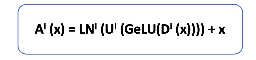
Where

x is a d dimensional input
LN^l is layer normalization for the lth Adapter layer
U^l is feed-forward up-project m * d weight matrix
D^l is feed forward down-project d * m weight matrix
GeLU : activation funciton
+ : residual connection

The bottleneck dimension, m, provides a simple means to trade-off performance with parameter efficiency. The adapter module itself has a skip-connection internally. With the skip-connection, if the parameters of the projection layers are initialized to near-zero, the module is initialized to an
approximate identity function. Alongside the layers in the adapter module, we also train new layer normalization parameters per task.

Pruning Adapters from lower layers

In [9] authors suggest that Adapters on the lower layers have a smaller impact than the higher-layers. Removing the adapters from the layers 0 − 4 on MNLI barely affects performance. Focusing on the upper layers is a popular strategy in fine-tuning. One intuition is that the lower layers extract lower-level features that are shared among tasks, while the higher layers build features that are unique to different tasks.

4. Adapters For Multi Task Learning

A key issue with multi-task fine-tuning is the potential for task interference or negative transfer, where achieving good performance on one task can hinder performance on another.

Common techniques to handle task interference are

Different learning rates for the encoder layer of each task
Different regularization schemes for task specific parameters e.g. Query Key Attention matrix normalization[11]
Tuning Task’s Weights In The Weighted loss function[12]

In [10] Ruder et. al. proposes an adapter based architecture for fine-tuning transformers in multi-task learning scenario. The authors introduces the concept of shared “hypernetwork“, that can learn adapter parameters for all layers and tasks by generating them using shared hyper networks, which condition on task, adapter position, and layer id in a transformer model. Instead of adding separate adapters for each task, [10] uses a “hypernetwork” to generate parameters for adapter’s feed forward down-project weight matrix and feed-forward up-project weight matrix.

*[10] Adapter Layers used for Multi Task fine tuning LLMs*

The above image shows how the Feed Forward(FF) matrices for the adapter modules are being generated from the hyper-network. For the Adapter in l^th layer, the FF down projection matrix is depicted by D^l and the the FF up project matrix is depicted as U^l.

[10] also introduces the idea of Task Embedding I_t that would be generated by another sub network and will be conditional on task specific input (imagine the task prompt here). This task embedding I_t will be used to generate each Task Adapter’s down projection matrix and up project matrix for each layer. Similarly, the layer normalization hyper-network h^l _LN generates the conditional layer normalization parameters (βτ and γτ ).

How to Generate Task Specific Adapter Matrices From Task Embedding?

The hyper-network learns to generate task and layer-specific adapter parameters, conditioned on task and layer id embeddings. The hyper-network is jointly learned between all tasks and is thus able to share information across them, while negative interference is minimized by generating separate adapter layers for each task. For each new task, the model only requires learning an additional task embedding, reducing the number of trained parameters.

The key idea is to learn a parametric task embedding {Iτ }^T_τ=1 for each task, and then feed these task embeddings to hyper-networks parameterized by ν that generate the task-specific adapter layers. Adapter modules are inserted within the layers of a pre-trained model.

For generating feed-forward up-project matrix U^l _T and feed forward down-project matrix D^l _T from task embedding I_t, we perform following operation

D^l_τ∈R^h×d : Down project matrix for task T

U^l_τ∈R^dxh : Up project matrix for task T

W^U, W^D : Learnable projection matrices

Here h is the input dimension, and d is the bottleneck dimension, the matrices W^U and W^D are learnt for each layer and they are task independent. We project the task embedding I_t to these matrices to generate the task specific FF up project and FF down project matrices. We consider simple linear layers as hyper-networks that are functions of input task embeddings Iτ.

5. LLaMA Adapters

“LLaMA Adapter is a lightweight adaption method to fine-tune LLaMA into an instruction following model” [13]. It uses the same 52K data points used by Alpaca[3] to fine tune 7B frozen Llama[2] model adding only 1.2M learnable parameters and taking only one hour on 8 A100 GPUs.

LLaMA Adapter got inspiration from two key ideas discussed earlier in this post.

Learnable Prompts: It adopt a set of learnable adaption prompts (like Prefix-tuning discussed in section 2), and prepend them to the input text tokens at higher transformer layers.
- Adapter’s added to only higher layers : Set of learnable adaption prompts were appended as prefix to the input instruction tokens in higher transformer layers. These prompts learn to adaptively inject new instructions (conditions) into LLaMA.
Zero-init attention : A zero-init attention mechanism with zero gating was used for the prompt embedding. A similar approach was taken by Parameter-Efficient Transfer Learning for NLP[9] by using Near-identity initialization for adapter FF up project and down project matrices (weights initialized from Normal distribution with 0 mean and standard deviation 10⁻²
- Stability during training: To avoid noise from adaption prompts at the early training stage, we modify the vanilla attention mechanisms at inserted layers to be zero-init attention, with a learnable gating factor.

For a N layer transformer LLaMa Adapter only adds learnable adaption prompts to top L layers and (L ≤ N).

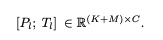
Adapter Prompt Tensor at l^th layer: {P^l}^L _l=1 where P^l ∈ R^K×C with K desnotes the prompt length for each layer, and C equals the feature dimension of LLaMA transformer.

Input Text Tensor at l^th layer: M-length word tokens are denoted as T^l∈ R^M×C

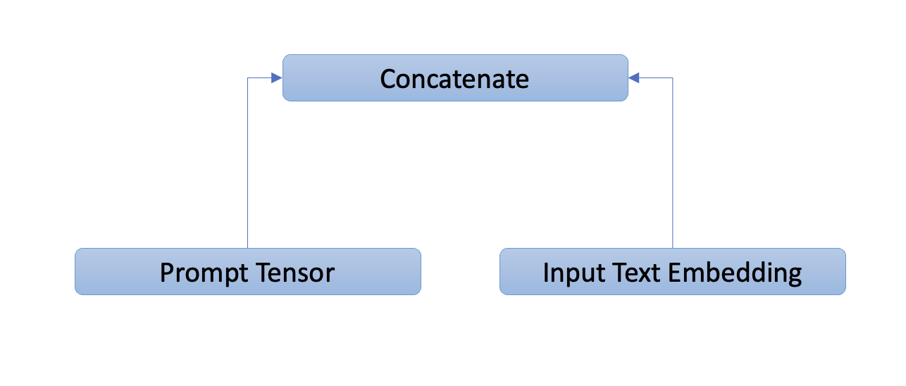
Final Prompt: The adaption prompt is concatenated with T^lalong the token dimension as prefix,

Hence instruction knowledge learned within P^l can effectively guide T^l to generate contextual responses.

[13] Adapter and Input Tokens Fusion In Top L layers

The above image shows that all N layers of the transformer are “frozen” and only Adapter comprise of learnable tensors (L learnable tensors, one for each of the top L layer). Furthermore while the transformer has vanilla attention layers, LLaMa adapters uses zero-init attention and gating mechanisms.

6. LORA: LOW-RANK ADAPTATION OF LARGE LAN-
GUAGE MODELS

LoRA[14] injects trainable rank decomposition matrices into each layer of the Transformer architecture thereby reducing the number of trainable parameters for downstream tasks. The parameters of the original pre-trained transformer remains frozen. LoRA drives intuition from Aghajanyan et.al [16] which shows that the learned over-parametrized models in fact reside on a low intrinsic dimension. This led to the hypothesis that change in weights during model adaptation also has a low “intrinsic rank”,

The paper further states that LoRA allows to train some dense layers in a neural
network indirectly by optimizing rank decomposition matrices of the dense layers’ change during
adaptation instead, while keeping the pre-trained weights frozen.

Low Rank Decomposition

In the above image a m x n weight W is decomposed into m x k matrix A and k x n matrix B. In linear algebra, the rank[16] of a matrix W is the dimension of the vector space generated by its columns. This corresponds to the maximal number of linearly independent columns of W. Over parametrized weight matrices can contain linearly dependent columns, hence they can be decomposed into product of smaller matrices.

One of the most popular method to perform low rank decomposition is Singular Value Decomposition[17].

For a m x n matrix M, SVD factorizes M into orthonormal matrices U and V. V* is the conjugate transpose of V. $\ \mathbf {\Sigma } \$ is a diagonal matrix with non-negative real numbers on the diagonal.

Calculating the SVD consists of finding the eigenvalues and eigenvectors of MM^Tand M^TM. The eigenvectors of M^TM make up the columns of V , the eigenvectors of MM^T make up the columns of U. Also, the singular values in $\ \mathbf {\Sigma } \$ are square roots of eigenvalues from MM^T or M^TM. For more details around calculating U, $\ \mathbf {\Sigma } \$ and V please check [18]. The number of non-zero singular values is equal to the rank of M

LoRA’s LOW-RANK-PARAMETRIZED UPDATE MATRICES

For a pre-trained weight matrix W₀∈ R^d×k LoRA constrains its update by representing the latter with a low-rank decomposition W₀ + ∆W = W₀ + BA, where B ∈ R^d×r, A ∈ R^r×k , the rank r min(d, k).

During training, W₀ is frozen and does not receive gradient updates, while A and B contain trainable parameters.

Note both W₀ and ∆W = BA are multiplied with the same input, and their respective output vectors are summed coordinate-wise. For h = W₀x, our modified forward pass yields:

h = W₀ x + ∆W x = W₀ x + BA x

Random Gaussian initialization is used to initialize matrix A and matrix B is initialized to zero, so ∆W = BA is zero at the beginning of training.

For GPT-3 175B, the authors set a parameter budget of 18M (in FP16), that corresponds to r=8 if they adapt one type of attention matrix (from Query, Key and Value matrix) or r = 4 if they adapt two types of attention matrices for all 96 layers of GPT 3.

Adapting both W_q and W_v gives the best performance overall.

LoRA’s Effect On Inference Latency

Adding Adapter layers sequentially between Transformer’s layers induces inference time latency. There is no direct ways to bypass the extra compute in adapter layers. This seems like a non-issue since adapter layers are designed to have few parameters (sometimes <1% of the original model) by having a small bottleneck dimension, which limits the FLOPs they can add. However, large neural networks rely on hardware parallelism to keep the latency low, and adapter layers have to be processed sequentially. This makes a difference in the online inference setting where the batch size is typically as small as one.

When deployed in production, LoRA can explicitly compute and store W = W₀ + BA and perform inference as usual. Note that both W₀ and BA are in R^d×k . LoRA has no effect on inference time latency.

Finding The Optimal rank r for LoRA

Although LoRA already performs competitively for low values of r (4 and 8 in the above example), a natural question to ask is what’s the optimal value for r given a weight matrix W?

The authors in [14] check the overlap of the subspaces learned by different choices of r and by different random seeds. They showed that increasing r does not cover a more meaningful subspace, which suggests that a low-rank adaptation matrix is sufficient.

Grassmann Distance[19]

Grassmann distance helps us measure subspace overlap or similarity between the subspace spanned by column vectors of two matrices. Now given two low rank decomposition

Given low rank projection of weight matrix A into A_r=8 and A_r=64 which are the learned adaptation matrices with rank r = 8 and 64 using the same pre-trained model, [14] performs singular value decomposition and obtain the right-singular unitary matrices U_Ar=8 and U_Ar=64. Then authors in [14]
ventured to answer the question, how much of the subspace spanned by the top i singular vectors in U_Ar=8 (for 1 ≤ i ≤ 8) is contained in the subspace spanned by top j singular vectors of U_Ar=64 (for 1 ≤ j ≤ 64).

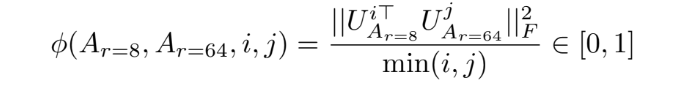
where Uⁱ_Ar=8 represents the columns of U_Ar=8 corresponding to the top-i singular vectors. φ(·) has a range of [0, 1], where 1 represents a complete overlap of subspaces and 0 a complete
separation. [14] shows that the top singular-vector directions of A_r=8and A_r=64 are the most useful, while other directions potentially contain mostly random noises accumulated during training. Hence, the adaptation matrix can indeed have a very low rank.

7. Code Pointers

Colab link to fine tune quantized (int 8) 6B parameter Llama with LoRa

Download Llama in int 8 format

import os
os.environ["CUDA_VISIBLE_DEVICES"]="0"
import torch
import torch.nn as nn
import bitsandbytes as bnb
from transformers import AutoTokenizer, AutoConfig, AutoModelForCausalLM

model = AutoModelForCausalLM.from_pretrained(
    "facebook/opt-6.7b", 
    load_in_8bit=True, 
    device_map='auto',
)
tokenizer = AutoTokenizer.from_pretrained("facebook/opt-6.7b")

Freeze model parameters and cast Layer Normalization and head to FP16 for stability during training (original model is in int 8)

for param in model.parameters():
  param.requires_grad = False  # freeze the model - train adapters later
  if param.ndim == 1:
    # cast the small parameters (e.g. layernorm) to fp32 for stability
    param.data = param.data.to(torch.float32)

model.gradient_checkpointing_enable()  # reduce number of stored activations
model.enable_input_require_grads()

class CastOutputToFloat(nn.Sequential):
  def forward(self, x): return super().forward(x).to(torch.float32)
model.lm_head = CastOutputToFloat(model.lm_head)

Apply LoRA PEFT wrapper to 8 bit Llama

from peft import LoraConfig, get_peft_model 

config = LoraConfig(
    r=16,
    lora_alpha=32,
    target_modules=["q_proj", "v_proj"],
    lora_dropout=0.05,
    bias="none",
    task_type="CAUSAL_LM"
)

model = get_peft_model(model, config)
print_trainable_parameters(model)

Here we are only adding adapters for Query and Value attention matrices. The rank parameter is 16.

The output shows that only .13% parameters of the 6.6 B parameter Llama model.

trainable params: 8388608 || all params: 6666862592 || trainable%: 0.12582542214183376

	Revamping Dual Encod… on Feature Fusion For The Un…
	Neural Ranking Archi… on Feature Fusion For The Un…
	Neural Ranking Archi… on Talk On Multi Stage Ranki…
	Graph Neural Network… on Attribute Discovery For E-Comm…
	Siddharth Sharma on CTR Prediction System –…