
~30% Compression Of LLM (Flan-T5-Base) With Low Rank Decomposition Of Attention Weight Matrices
Colab Link To Reproduce Experiment: LLM Compression Via Low Rank Decomposition.ipynb
Context
A neural network contains many dense layers which perform matrix multiplication. In the case of Transformers, Attention module has Key, Query, Value and Output matrices (along with the FF layer) that are have typically full rank. Li. et al. [3] and Aghajanyan et al.[4] shows that the learned over-parametrized models in fact reside in low intrinsic dimension. In popular Parameter Efficient Fine Tuning(PEFT) technique LoRA, the authors took inspiration from [3] and [4] to hypothesize that the change in weights during model adaptation also has a low intrinsic rank.
In real production models, the model capacity is often constrained by limited serving resources and strict latency requirements. It is often the case that we have to seek methods to reduce cost while
maintaining the accuracy. To tame inference time latency, low rank decomposition of weight matrices have earlier been used in applications like DCN V2[5].
Low Rank Decomposition
Low rank decomposition of a dense matrix 𝑀 ∈ R𝑑×𝑑 by two tall and skinny matrices
𝑈 ,𝑉 ∈ R𝑑×𝑟 helps us approximate M by only using U and V (way less parameters than original matrix M). Here r << d.

In the above image a m x n weight W is decomposed into m x k matrix A and k x n matrix B. In linear algebra, the rank[6] of a matrix W is the dimension of the vector space generated by its columns. This corresponds to the maximal number of linearly independent columns of W. Over parametrized weight matrices can contain linearly dependent columns, hence they can be decomposed into product of smaller matrices.
One of the most popular method to perform low rank decomposition is Singular Value Decomposition[7].
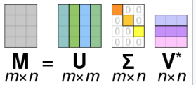
For a m x n matrix M, SVD factorizes M into orthonormal matrices U and V. V* is the conjugate transpose of V. 
Calculating the SVD consists of finding the eigenvalues and eigenvectors of MMT and MTM. The eigenvectors of MTM make up the columns of V , the eigenvectors of MMT make up the columns of U. Also, the singular values in
In this post I further explore effects of taking low rank decomposition of attention weight matrices (Query, Key, Value and Output) on T5-base performance.
Spectrum Decay
This section plots the Singular values of Query matrix of last decoder layer of flan-base (~220 million params) and flan-large (~700 million params) models.
Flan Base Weight Matrix (768 x 768)  = decoder.block[11].layer[0].SelfAttention.q.weight

Flan Large Weight Matrix (1024 x 1024) = decoder.block[23].layer[0].SelfAttention.q.weight
The above plot shows the singular value decay pattern of the learned weight matrices from flan-t5-base and flan-t5-large. The above plot shows a much faster spectrum decay pattern than a linear decline, reinforcing our hypothesis that Large Language Models have intrinsic low rank.

The above plot shows Frobenius norm of difference between attention Query weight matrix of decoder’s last layer and it’s approximation from low rank decomposition (r varies from 32 to 768 for flan-t5-base and 32 to 1024 for flan-t5-large)
Low Rank Layers
The Low Rank Layer creates SVD of weight matrix of attention matrices of original model. Then we use a configurable parameter “r” to decide the rank of matrix to use.
Config to choose rank and targeted params
@dataclass
class LowRankConfig:
    rank:int
    target_modules: list[str]

#low rank decomposition of SelfAttention Key, Query and Value Matrices
config = LowRankConfig(
    rank= 384,
    target_modules=["k", "q", "v", "o"]
)
Code pointer creating low rank layers
The module below accepts a full rank layer (we experimented with Linear Layers) and rank parameter “r”. It performs SVD of the weight matrix and then save the low rank matrices U, S and Vh.
This module can be further optimized by precomputing product of U and S or S and Vh.
class LowRankLayer(nn.Module):
    """given a linear layer find low rank decomposition"""
    def __init__(self, rank, full_rank_layer):
        super().__init__()
        self.rank = rank
        U, S, Vh = torch.linalg.svd(full_rank_layer.weight)
        S_diag = torch.diag(S)
        self.U = U[:, :self.rank]
        self.S = S_diag[:self.rank, :self.rank]
        self.Vh = Vh[:self.rank, :]

    def forward(self, x):
        aprox_weight_matrix = self.U @ self.S @ self.Vh
        output = F.linear(x, aprox_weight_matrix)
        return output
After this step we replaces the targeted layers with the new Low Rank Layers.
Effect On Model Size
| Model Name | #Params | Rank | Target Modules | |
| google/flan-t5-base | 247577856 | 382 | NA | |
| Low Rank – google/flan-t5-base | 183876864 | 382 | [“q”, “k”, “v”] | |
| Low Rank – google/flan-t5-base | 162643200 | 382 | [“q”, “k”, “v”, “o”] | |
Projecting Random Vectors
An intuitive way to see the effect of low rank approximation technique is to project a random vector (input) on the original matrix and the one created from low rank approximation
#low rank approximation of model_t5_base.encoder.block[0].layer[0].SelfAttention.q
# 768 to 384 dim reduction
query_attention_layer = model_t5_base.encoder.block[0].layer[0].SelfAttention.q
low_rank_query_attention_layer = LowRankLayer(384, model_t5_base.encoder.block[0].layer[0].SelfAttention.q)
Now we would find projection of the random 768 length tensor on query_attention_layer and low_rank_query_attention_layer
random_vector = torch.rand(768)
low_rank_projection = low_rank_query_attention_layer(random_vector)
original_projection = query_attention_layer(random_vector)
Now we would find Cosine Similarity between the two vectors
cosine_sim = torch.nn.CosineSimilarity(dim=0)
cosine_sim(low_rank_projection, original_projection)Output: tensor(0.9663, grad_fn=<SumBackward1>)
This show that the effect of original Query matrix and its low rank approximation on a random input is almost same.
Evaluation
In this section we compare performance of low rank approximation on performance w.r.t Summarization Task (Samsum data set)
| Model | eval_loss | eval_rogue1 | eval_rouge2 | eval_rougeL | eval_rougeLsum |
| flan-t5-large | 1.467 | 46.14 | 22.31 | 33.58 | 42.13 |
| compressed model | 1.467 | 46.11 | 22.35 | 38.57 | 42.06 |
As we can see from the above table, there is almost no drop in performance of the compressed model on summarization task.
References
- LoRA: Low-Rank Adaptation of Large Language Models
- Learning Low-rank Deep Neural Networks via Singular Vector Orthogonality Regularization and Singular Value Sparsification
- Measuring the Intrinsic Dimension of Objective Landscapes
- Intrinsic Dimensionality Explains the Effectiveness of Language Model Fine-Tuning
- DCN V2: Improved Deep & Cross Network and Practical Lessons for Web-scale Learning to Rank Systems
- https://en.wikipedia.org/wiki/Rank_(linear_algebra)
- https://en.wikipedia.org/wiki/Singular_value_decomposition
- https://web.mit.edu/be.400/www/SVD/Singular_Value_Decomposition.htm
Posted in Large Language Models, llm, machine learning
Tagged large language model, machine learning
Leave a comment
Adapter Based Fine Tuning BART And T5-Flan-XXL For Single Word Spell Correction
In this post I share results of a weekend project around fine tuning BART and T5 Flan models for sequence to sequence generation. I have used common misspellings in English language (single words) for training and evaluating the models. As a benchmark I have first trained and evaluated a pre-trained checkpoint of BART and then followed with LoRA based fine-tuning for BART and Flan T5 XXL.
Data set used: Peter Norvig’s Common English Misspellings Data Set
Model Type : AutoModelForSeq2SeqLM
PEFT Task Type: SEQ_2_SEQ_LM
| Model | Colab Code Pointers | Checkpoint | PEFT Type | #Params | #Trainable-Params | |
| BART | bart-seq-2-seq | “facebook/bart-base” | NA (full model fine tuning) | 255 million | 255 million | |
| BART | bart-lora | “facebook/bart-base” | LoRA | 255 million | 884.7k (0.41%) | |
| BART | bart-8bit-lora | “facebook/bart-base” – 8 bit | LoRA | 255 million | 884.7k (0.41%) | |
| T5-Flan-XXL | t5-flan-xxl-lora | “philschmid/flan-t5-xxl-sharded-fp16” – 8 bit | LoRA | ~11.15 billion | 18.87 Milion (0.17%) | |
BART VS T5
Bart[1] and T5[2] are both have Seq2Seq[3] model architecture. They both uses Encoder-Decoder style architecture, where Encoder is like BERT’s encoder and Decoder is autoregressive. Essential it is a de-noising auto-encoder that maps a corrupted document to the original document (using an auto-regressive decoder).
BART uses a variety of input text corruption mechanism and a Seq2Seq model to reconstruct output. Bart’s authors evaluated a number of noising approaches for pre-training e.g.

- Token Masking: Random tokens are sampled and replaced with [MASK]
- Token Deletion – Random tokens are deleted from the input. This helps model lean which positions are missing input.
- Text Infilling: A number of text spans are sampled with span lengths drawn from a Poisson distribution. Each span is replaced with a single [MASK] token. Text Infilling is inspired from SpanBERT. It teaches the model to predict how many tokens are missing from a span.
- Sentence Permutation: A document is divided into sentences based on full stops and these sentences are shuffled at random.
- Document Rotation : A token is chosen uniformly at random and the document is rotated so that it begins with that token.
T5-Flan has same number of parameters as T5(Text-to-Text Transfer Transformer) but it is fine-tuned on more than 1000 additional tasks covering also more languages.
| #Layers | #Parameters | Vocab Size | Embedding Size | ||
| BART-Base | 6 Encoder 6 Decoder | 255 million | ~50k | 1024 | |
| T5-Large | 14 Encoder 14 Decoder | 780 million | ~32k | 4096 | |
| T5-Flan-XXl | 23 Encoder (T5 Blocks) 23 Decoder (T5 Blocks) | 11.15 Billion | ~32k | 4096 |
T5 Model has following Modules (Huggingface implementation 8-bit checkpoint)
a. Shared Embedding Layer (Encoder and Decoder modules share this layer) of size (32128, 4096)
b. Encoder T5 Block – Attention Layer and Feed Forward Layer
T5Block(
        (layer): ModuleList(
          (0): T5LayerSelfAttention(
            (SelfAttention): T5Attention(
              (q): Linear8bitLt(in_features=4096, out_features=4096, bias=False)
              (k): Linear8bitLt(in_features=4096, out_features=4096, bias=False)
              (v): Linear8bitLt(in_features=4096, out_features=4096, bias=False)
              (o): Linear8bitLt(in_features=4096, out_features=4096, bias=False)
              (relative_attention_bias): Embedding(32, 64)
            )
            (layer_norm): T5LayerNorm()
            (dropout): Dropout(p=0.1, inplace=False)
          )
          (1): T5LayerFF(
            (DenseReluDense): T5DenseGatedActDense(
              (wi_0): Linear8bitLt(in_features=4096, out_features=10240, bias=False)
              (wi_1): Linear8bitLt(in_features=4096, out_features=10240, bias=False)
              (wo): Linear(in_features=10240, out_features=4096, bias=False)
              (dropout): Dropout(p=0.1, inplace=False)
              (act): GELUActivation()
            )
            (layer_norm): T5LayerNorm()
            (dropout): Dropout(p=0.1, inplace=False)
          )
        )
c. Decoder T5 Blocks –
i. Self Attention Layer
ii. Cross Attention Layer
iii. Feed Forward Layer
T5Block(
        (layer): ModuleList(
          (0): T5LayerSelfAttention(
            (SelfAttention): T5Attention(
              (q): Linear8bitLt(in_features=4096, out_features=4096, bias=False)
              (k): Linear8bitLt(in_features=4096, out_features=4096, bias=False)
              (v): Linear8bitLt(in_features=4096, out_features=4096, bias=False)
              (o): Linear8bitLt(in_features=4096, out_features=4096, bias=False)
              (relative_attention_bias): Embedding(32, 64)
            )
            (layer_norm): T5LayerNorm()
            (dropout): Dropout(p=0.1, inplace=False)
          )
          (1): T5LayerCrossAttention(
            (EncDecAttention): T5Attention(
              (q): Linear8bitLt(in_features=4096, out_features=4096, bias=False)
              (k): Linear8bitLt(in_features=4096, out_features=4096, bias=False)
              (v): Linear8bitLt(in_features=4096, out_features=4096, bias=False)
              (o): Linear8bitLt(in_features=4096, out_features=4096, bias=False)
            )
            (layer_norm): T5LayerNorm()
            (dropout): Dropout(p=0.1, inplace=False)
          )
          (2): T5LayerFF(
            (DenseReluDense): T5DenseGatedActDense(
              (wi_0): Linear8bitLt(in_features=4096, out_features=10240, bias=False)
              (wi_1): Linear8bitLt(in_features=4096, out_features=10240, bias=False)
              (wo): Linear(in_features=10240, out_features=4096, bias=False)
              (dropout): Dropout(p=0.1, inplace=False)
              (act): GELUActivation()
            )
            (layer_norm): T5LayerNorm()
            (dropout): Dropout(p=0.1, inplace=False)
          )
        )
Tokenization
For BART we follow standard sequence to sequence tokenization scheme. In the example below we tokenize input text and label text.
def bart_preprocess_function(sample,padding="max_length"):

    # tokenize inputs
    model_inputs = tokenizer(sample["misspelled_queries"], max_length=max_source_length, padding=padding, truncation=True)

    # Tokenize targets with the `text_target` keyword argument
    labels = tokenizer(text_target=sample["correct_spelling"], max_length=max_target_length, padding=padding, truncation=True)

    model_inputs["labels"] = labels["input_ids"]
    return model_inputs
Where as for T5-Flan-XXL we would have to append the input text with a context prompt
def t5_preprocess_function(sample, max_source_length = 12, max_target_length= 12, padding="max_length"):
    # add prefix to the input for t5
    inputs = ["correct spelling of following word : " + item for item in sample["misspelled_queries"]]

    # tokenize inputs
    model_inputs = tokenizer(inputs, max_length=max_source_length, padding=padding, truncation=True)

    # Tokenize targets with the `text_target` keyword argument
    labels = tokenizer(text_target=sample["correct_spelling"], max_length=max_target_length, padding=padding, truncation=True)

    # If we are padding here, replace all tokenizer.pad_token_id in the labels by -100 when we want to ignore
    # padding in the loss.
    if padding == "max_length":
        labels["input_ids"] = [
            [(l if l != tokenizer.pad_token_id else -100) for l in label] for label in labels["input_ids"]
        ]

    model_inputs["labels"] = labels["input_ids"]
    return model_inputs
Adapter Based Fine-tuning
Once we have downloaded an 8 bit model checkpoint we use LoRA adapter from Huggingface PEFT module and use it as a wrapper
from peft import LoraConfig, get_peft_model, prepare_model_for_int8_training, TaskType

# Define LoRA Config
lora_config = LoraConfig(
 r=16,
 lora_alpha=32,
 target_modules=["q", "v"], # for BART use ["q_proj", "v_proj"]
 lora_dropout=0.05,
 bias="none",
 task_type=TaskType.SEQ_2_SEQ_LM
)
# prepare int-8 model for training
model = prepare_model_for_int8_training(model) #skip this for BART

# add LoRA adaptor
model = get_peft_model(model, lora_config)
model.print_trainable_parameters()
32 bit checkpoint vs 8 bit checkpoint
I also tried comparing performance of PEFT Bart with 32 bit checkpoint as well as 8 bit checkpoint. The results were almost comparable, although inferencing on 8 bit checkpoint was reasonably faster.
Additional improvements for 8 bit check point involved using FP16 for layernorm layers and FP32 for the LM head for model stability during training.
import torch
for param in model.parameters():
  # param.requires_grad = False  # freeze the model - train adapters later
  if param.ndim == 1:
    # cast the small parameters (e.g. layernorm) to fp32 for stability
    param.data = param.data.to(torch.float16)

# model.gradient_checkpointing_enable()  # reduce number of stored activations
# model.enable_input_require_grads()

class CastOutputToFloat(nn.Sequential):
  def forward(self, x): return super().forward(x).to(torch.float32)
model.lm_head = CastOutputToFloat(model.lm_head)
A recalcitrant issue was with using gradient_checkpointing with the above approach. If I remember it correctly somehow Huggingface Trainer API throw following error.
Performance Results (Test Data)
The table below shows performance of different fine-tuned models w.r.t. misspelled query and corrected spelling edit distance.
| Edit-Distance | Accuracy Bart | Accuracy Bart – LoRA | Accuracy Bart 8 bit – LoRA | Accuracy T5-Flan-XXL – LoRA | |||
| 1 | 49.34 | 32.12 | 31.79 | 53.79 | |||
| 2 | 52.55 | 18.82 | 18.82 | 42.75 | |||
| 3 | 48.60 | 14.04 | 14.02 | 35.51 | |||
| 4 | 48.76 | 11.57 | 12.40 | 33.88 | |||
| 5 | 27.27 | 5.45 | 3.64 | 12.73 | |||
| 6 | 39.39 | 9.09 | 9.09 | 18.18 |
References
- BART: Denoising Sequence-to-Sequence Pre-training for Natural Language Generation, Translation, and Comprehension
- Exploring the Limits of Transfer Learning with a Unified Text-to-Text Transformer
- Sequence to Sequence Learning with Neural Networks
- T5-Flan : Scaling Instruction-Finetuned Language Models
Posted in Uncategorized
Tagged large language model, llm, lora, machine learning, nlp, spell correction
Leave a comment
Revamping Dual Encoder Model Architecture: A layered approach to fuse multi-modal features and plug-and-play integration of Encoders
Code examples of feature fusion techniques and tower encoders in last half of the blog

In Embedding Based Retrieval(EBR) we create embedding of search query in an online manner and then find k-nearest neighbors of the query vector in an index of our entity embeddings (e.g. E-Commerce product, legal/medical document, Linkedin/Tinder user profile, Music, Podcast, Playlist etc). The query and entity embeddings are learnt from a model based on contrastive learning. While query is normally short text, the matched entity has rich feature space (text, float features, image etc). Irrespective of the business problem and model architecture followed (dual encoder, late interaction etc.), a common challenge faced while developing contrastive learning models is how to encode and fuse features of different modalities to create unified representation of an entity and then transform that using some encoder.
Types Of Retrieval Model Architectures

Dual Encoder or Bi-Encoder [1] architecture creates two tower architecture, where the towers correspond to query embedding encoder and Entity embedding encoder. Finally the similarity between the transformed embeddings are calculated and contrastive loss[2] is used to learn the encoder parameters.
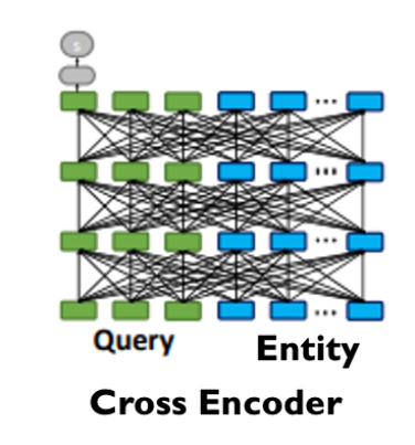
Cross Encoders are Bert[3] or Roberta[4] Encoder style network that performs attention based early fusion between query and entity feature embedding. Although this architecture performs better in similarity tasks (e.g. sentence similarity[5]), due to early fusion these encoders are computationally heavy and inference latency is on the higher end compared to dual encoder based architecture. Due to high inference time latency these encoders are not suited when the candidate set to be compared with query vector is large.
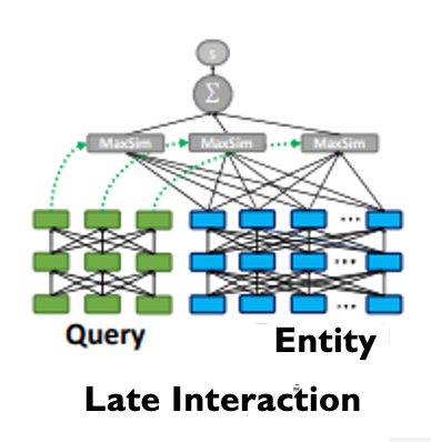
ColBERT[6] adapts deep Language Models (in particular, BERT) for efficient retrieval. ColBERT introduces a late interaction architecture that independently encodes the query and the document using BERT and then employs a cheap yet powerful interaction step that models their fine-grained similarity. By delaying and yet retaining this granular interaction, ColBERT can leverage the expressiveness of deep Language Models while simultaneously gaining the ability to pre-compute document representations cosine, considerably speeding up query processing.
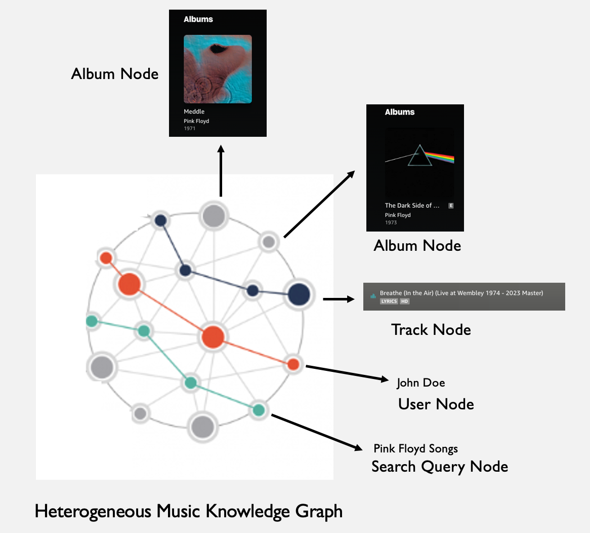
In heterogeneous graphs like the above music graph, we can use graph convolution[7][8] to learn node embeddings based on its local neighborhood.
Generating Initial Entity Embedding From Features
A common problem in all four architectures is how to generate initial entity embedding from its multi modal features. Whether it is e-commerce product, user profile on social media, music track on Amazon Music, a precursor to choosing the model architecture is how to fuse their features together to generate entity embedding (node embedding in the case of graph). Once we have the initial entity representation then we can fine tune it using the architectures discussed above.
How to process and fuse these features to generate unified music album embedding to feed to the entity tower network?

High Level Architecture
Architecture Type : Two Tower / Dual Encoder

1. Input Layer
The input layer will ingest data in the following format.

The above schema helps to standardize the input format and make it agnostic of the domain i.e. whether it is music song, e-commerce product or social media user profile, the features can be stored using the same schema. Features are grouped based on their semantic structure (data type) e.g. all embedding based features will be in embedding_features_map where key would be feature_id/feature_name and value would be feature’s corresponding embedding (float vector).
Types Of Features
- Dense Features
- float value features
- e.g. ctr, number of clicks, frequency of queries etc
- dense_features_map will contain a dictionary where feature is key and corresponding float value will be used as dictionary value
- Category Features
- id based features
- e.g. category id, topic id, user id, podcast id etc
- category_id_features_map will contain feature id is key and corresponding id as value
- Embedding Based Features
- 1 D vector of float values
- e.g. thumbnail image embedding, title embedding, artist/author embedding
- embedding_features_map will be a dictionary of feature id (key) and corresponding vector of floats
- Id List Based Features
- List of ids features
- e.g.
- list of ids of last k songs listened by a user in last ‘x’ hours
- list of ids of last k topics searched by users in last ‘y’ days
- id_list_features_map will be a dictionary of feature id (key) and corresponding list of ids
- [Optional] String Based Features
- string values
- e.g. title, description etc
- string_features_map will be a dictionary of feature id (key) and string as a value
Input layer Module will perform following features
- IO : read input data from s3 or database tables (e.g. Hive or Redshift table)
- Sanity Checks And Validations: e.g. no duplicate feature ids as keys in the input feature maps, data type validations (embedding based features should be float vectors)
- convert the raw data (string, float, vector of floats etc) to respective torch Tensor objects
- Create Dataset and DataLoader objects
2. Feature Encoder Layer
In this layer of the network we would perform pre-processing (standardization, normalization of text and dense features) as well as transform each feature to a vector of floats i.e. their dense representations. This layer would extract features from input layer and transform them using custom encoders (more on that later in this section). Each feature would be encoded separately using end user’s choice of encoder.
Features Of Feature Encoder Layer
- Numerical features scaling, normalization and standardization
- Initialize Embedding matrices (new embeddings to be learned from categorical and id_list_features)
- Encoders
- These will be off the shelf Modules (pre-trained models or learnable PyTorch modules) to transform input features
- e.g. Frozen Bert, SentenceBert, Roberta etc to encode string features to dense representations
- Learnable MLP Encoders to encode dense features or transform other input representations (e.g. transform input embedding feature)
Examples:
Dense Feature Transform
- scale features between 0-1
- Add MLP Encoder (Full connected layer + Non Linearity) to transform dense input features to a fixed length representation
- In the diagram below dense features (integer and float value features) can be
- Music Track popularity
- In the diagram below dense features (integer and float value features) can be
- recency score
- completion rate
- #listens in last k days


String Features Transforms
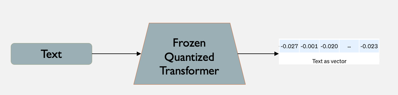
- Given text features we can create representations of text features using pre-trained transformers
- e.g. Text Sequence Encoder (we can make it configurable to use Bert, SentenceBert, Roberta, XLMR etc transformers)

One Hot Encoder:
Genre Encoder or Categorical Encoder : To encode “|” genres into one hot vectors

Identity Encoder
Convert features to Tensors

Categorical Embedding Encoder
- Song Genre to embedding
- Music Band/Artist embedding

Similarly we would have encoders for creating embeddings from categorical ids and id list based features by performing embedding lookup (trainable embedding matrices)
3. Feature Fusion Layer
In this layer we would use custom PyTorch modules to standardize pre-processing of different types of features. This would help ML engineers and Data scientists to speed up model development by using off the shelf boilerplate feature fusion modules.
For details into Feature Fusion please check my earlier blog on Feature Fusion For The Uninitiated
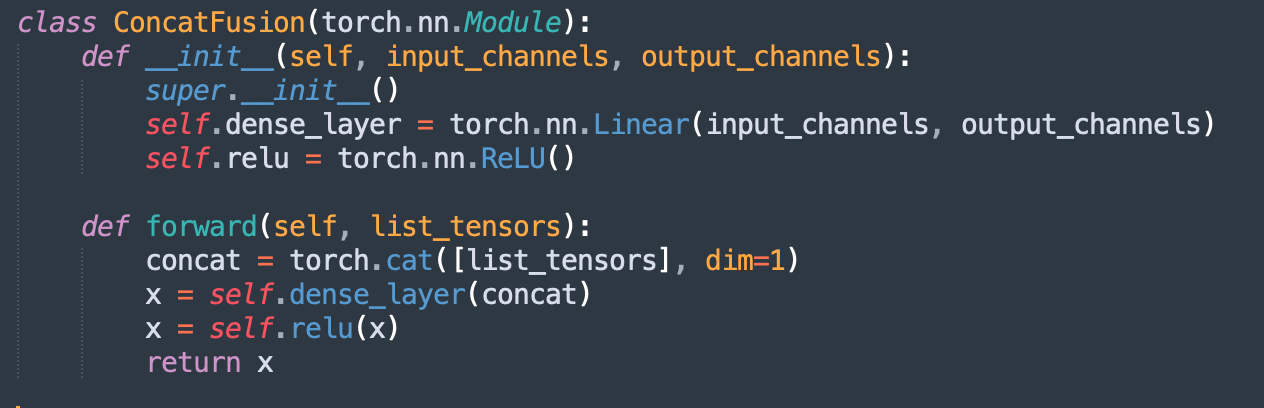
A. ConcatFusion: Concatenate And Transform
- vector-1 : Music Track title text embedding
- vector-2 : Album Embedding
- vector-3: Music Artist embedding

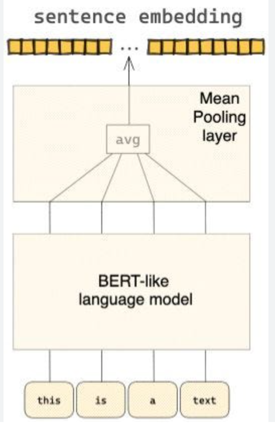
B. PoolingTransform
-
- In pooling transform once you have multiple feature embeddings (of equal length), you perform mean or max pooling to fuse them into one embedding (representing the entity)

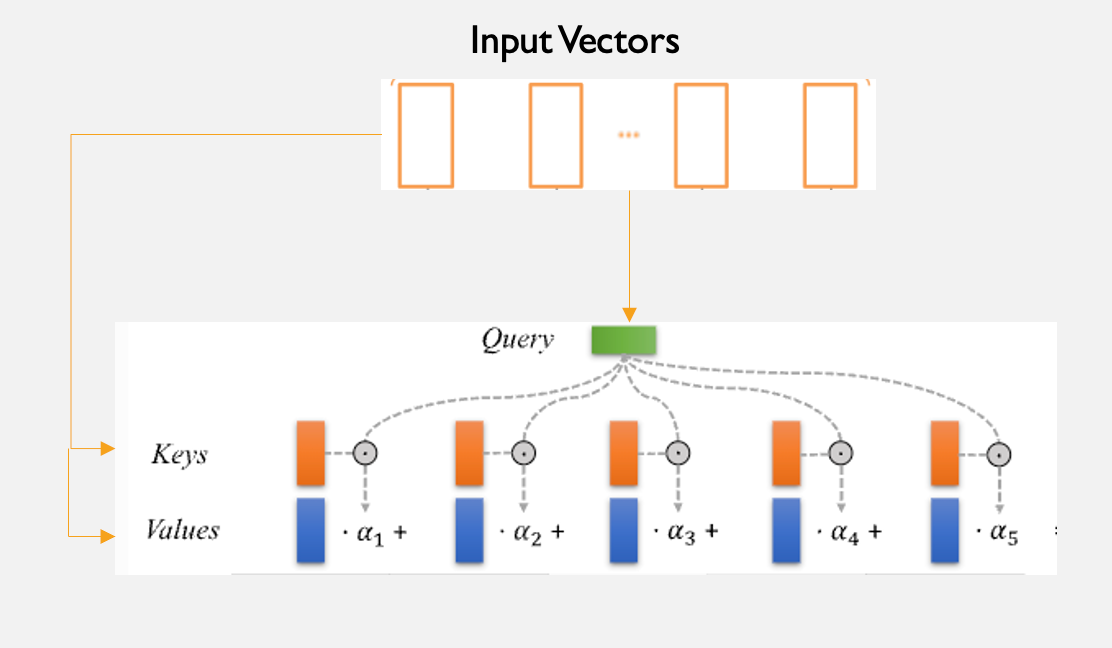
C. AttentionFusion
Attention based fusion applied multi headed attention[9] to the concatenated features vectors.

4.Encoder Layer
In this layer we would provide various kind of encoders that can be easily plugged in the proposed architecture. Query Encoder and Entity encoder will further process the output of feature fusion layer (a single embedding vector).
Some examples of Query/Entity Encoders can be
MLPEncoderTower

class MLPEncoderTower(nn.Module):
    def __init__(self, input_dims, number_of_mlp_layers):
        super().__init__()
        self.mlp_layers = nn.ModuleList(
        [MLPEncoder(input_dims, input_dims) for i in range(number_of_mlp_layers)]
        )

    def forward(self, x):
        for mlp_layer in self.mlp_layers:
            x = mlp_layer(x)
        return x
BertEncoderTower
from transformers import BertModel

class BertEncoderTower(nn.Module):
    def __init__(self):
        super().__init__(device = "cpu", num_layers)
        assert num_layers > 0, "number of encoder layers should be greater than 0"
        # encoder has only 12 layers
        num_layers = min(num_layers, 12)
        model = BertModel.from_pretrained("bert-base-uncased")
        self.encoder_layers = torch.nn.ModuleList(model.bert.encoder.layer[-num_layers:]).to(device)

    def forward(x):
        for attention_layer in self.encoder_layers:
            x = attention_layer(x)
References
- A Deep Relevance Matching Model for Ad-hoc Retrieval
- https://lilianweng.github.io/posts/2021-05-31-contrastive/
- BERT: Pre-training of Deep Bidirectional Transformers for Language Understanding
- RoBERTa: A robustly optimized BERT pretraining approach
- https://www.sbert.net/examples/applications/cross-encoder/README.html
- ColBERT: Efficient and Effective Passage Search via Contextualized Late Interaction over BERT
- Thomas N Kipf and Max Welling. 2017. Semi-supervised classification with graph convolutional networks. In ICLR.
- Will Hamilton, Zhitao Ying, and Jure Leskovec. 2017. Inductive representation learning on large graphs. In NIPS. 1024–1034.
- Attention is all you need
Posted in Uncategorized
Leave a comment
Summary Of Adapter Based Performance Efficient Fine Tuning (PEFT) Techniques For Large Language Models
The two most common transfer learning techniques in NLP were feature-based transfer (generating input text embedding from a pre-trained large model and using it as a feature in your custom model) and fine-tuning (fine tuning the pre-trained model on custom data set). It is notoriously hard to fine tune Large Language Models (LLMs) for a specific task on custom domain specific dataset. Given their enormous size (e.g. GPT3 175B parameters , Google T5 Flan XXL [1] 11B parameters, Meta Llama[2] 65 billion parameters) ones needs mammoth computing horsepower and extremely large scale datasets to fine tune them on a specific task. Apart from the mentioned challenges, fine tuning LLMs on specific task may lead them to “forget” previously learnt information, a phenomena known as catastrophic forgetting.
In this blog I will provide high level overview of different Adapter[4] based parameter efficient fine tuning techniques used to fine tune LLMs. PEFT based methods make fine-tuning large language models feasible on consumer grade hardware using reasonably small datasets, e.g. Alpaca[3] used 52 k data points to fine tune Llama 7B parameter model on multiple tasks in ~3 hours using a Nvidia A100 GPU[5].
HuggingFace PEFT module has 4 types of performance efficient fine-tuning methods available under peft.PEFT_TYPE_TO_CONFIG_MAPPING
{
'PROMPT_TUNING': peft.tuners.prompt_tuning.PromptTuningConfig,
 'PREFIX_TUNING': peft.tuners.prefix_tuning.PrefixTuningConfig,
 'P_TUNING': peft.tuners.p_tuning.PromptEncoderConfig,
 'LORA': peft.tuners.lora.LoraConfig
}
In this post I would go over theory of PROMPT_TUNING, PREFIX_TUNING and Adapter based techniques including LORA.
Before we dive into nitty-gritty of Adapter based techniques, let’s do a quick walkthrough of some other popular Additive fine tuning methods. “The main idea behind additive methods is augmenting the existing pre-trained model with extra parameters or layers and training only the newly added parameters.”[6]
1. Prompt Tuning
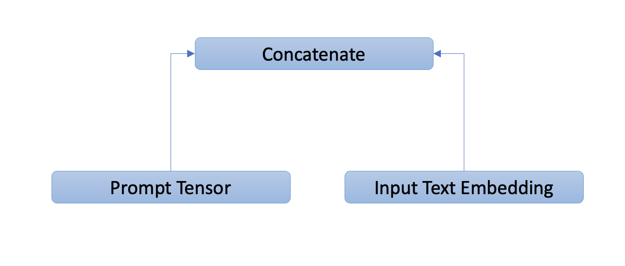
Prompt tuning[7] prepends the model input embeddings with a trainable tensor (known as “soft prompt”) that would learn the task specific details. The prompt tensor is optimized through gradient descent. In this approach rest of the model architecture remains unchanged.

2. Prefix-Tuning
Prefix Tuning is a similar approach to Prompt Tuning. Instead of adding the prompt tensor to only the input layer, prefix tuning adds trainable parameters are prepended to the hidden states of all layers.
Li and Liang[8] observed that directly optimizing the soft prompt leads to instabilities during training. Soft prompts are parametrized through a feed-forward network and added to all the hidden states of all layers. Pre-trained transformer’s parameters are frozen and only the prefix’s parameters are optimized.

3. Overview Of Adapter Based Methodology
What are Adapters ?
As an alternative to Prompt[7] and Prefix[8] fine tuning techniques, in 2019 Houlsby et.al.[9] proposed transfer learning with Adapter modules. “Adapter modules yield a compact and extensible model; they add only a few trainable parameters per task, and new tasks can be added without revisiting previous ones. The parameters of the original network remain fixed, yielding a high degree of parameter sharing.”[9]. Adapters are new modules added between layers of a pre-trained network. In Adapter based learning only the new parameters are trained while the original LLM is frozen, hence we learn a very small proportion of parameters of the original LLM. This means that the model has perfect memory of previous tasks and used a small number of new parameters to learn the new task.
In [9], Houlsby et.al. highlights benefits of Adapter based techniques.
- Attains high performance
- Permits training on tasks sequentially, that is, it does not require simultaneous access to all datasets
- Adds only a small number of additional parameters per task.
- Model retains memory of previous tasks (learned during pre-training).
Tuning with adapter modules involves adding a small number of new parameters to a model, which
are trained on the downstream task. Adapter modules perform more general architectural modifications to re-purpose a pre-trained network for a downstream task. The adapter tuning strategy involves injecting new layers into the original network. The weights of the original network are untouched, whilst the new adapter layers are initialized at random.
Adapter modules have two main features:
- A small number of parameters
- Near-identity initialization.
- A near-identity initialization is required for stable training of the adapted model
- By initializing the adapters to a near-identity function, original network is unaffected when training starts. During training, the adapters may then be activated to change the distribution of activations throughout the network.
Adapter Modules Architecture

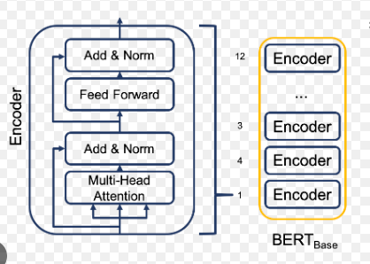
Two serial adapters modules are inserted after each of the transformer sub-layers (Attention and Feed Forward Layers). The adapter is always applied directly to the output of the sub-layer, after the projection back to the input size, but before adding the skip connection back. The output of the adapter is then passed directly into the following layer normalization.
How Adapters Minimize Adding New Parameters?
Down Project And Up Project Matrices
Adapter modules creates a bottleneck architecture where the adapters first project (feed forward down-project weight matrix in the above image) the original d-dimensional features into a smaller dimension, m, apply a nonlinearity, then project back (feed-forward up-project weight matrix) to d dimensions. The total number of parameters added per layer, including biases, is 2m*d + d + m. By setting m << d, the number of parameters added per task are limited (less than 1%).
Given an input x, the Adapter modules output at layer l would be
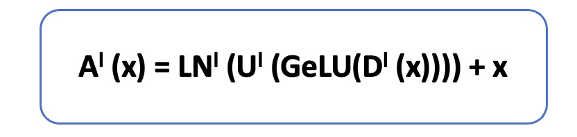
Where
- x is a d dimensional input
- LNl is layer normalization for the lth Adapter layer
- Ul is feed-forward up-project m * d weight matrix
- Dl is feed forward down-project d * m weight matrix
- GeLU : activation funciton
- + : residual connection
The bottleneck dimension, m, provides a simple means to trade-off performance with parameter efficiency. The adapter module itself has a skip-connection internally. With the skip-connection, if the parameters of the projection layers are initialized to near-zero, the module is initialized to an
approximate identity function. Alongside the layers in the adapter module, we also train new layer normalization parameters per task.
Pruning Adapters from lower layers
In [9] authors suggest that Adapters on the lower layers have a smaller impact than the higher-layers. Removing the adapters from the layers 0 − 4 on MNLI barely affects performance. Focusing on the upper layers is a popular strategy in fine-tuning. One intuition is that the lower layers extract lower-level features that are shared among tasks, while the higher layers build features that are unique to different tasks.
4. Adapters For Multi Task Learning
A key issue with multi-task fine-tuning is the potential for task interference or negative transfer, where achieving good performance on one task can hinder performance on another.
Common techniques to handle task interference are
- Different learning rates for the encoder layer of each task
- Different regularization schemes for task specific parameters e.g. Query Key Attention matrix normalization[11]
- Tuning Task’s Weights In The Weighted loss function[12]
In [10] Ruder et. al. proposes an adapter based architecture for fine-tuning transformers in multi-task learning scenario. The authors introduces the concept of shared “hypernetwork“, that can learn adapter parameters for all layers and tasks by generating them using shared hyper networks, which condition on task, adapter position, and layer id in a transformer model. Instead of adding separate adapters for each task, [10] uses a “hypernetwork” to generate parameters for adapter’s feed forward down-project weight matrix and feed-forward up-project weight matrix.

The above image shows how the Feed Forward(FF) matrices for the adapter modules are being generated from the hyper-network. For the Adapter in lth layer, the FF down projection matrix is depicted by Dl and the the FF up project matrix is depicted as Ul.
[10] also introduces the idea of Task Embedding It that would be generated by another sub network and will be conditional on task specific input (imagine the task prompt here). This task embedding It will be used to generate each Task Adapter’s down projection matrix and up project matrix for each layer. Similarly, the layer normalization hyper-network hl LN generates the conditional layer normalization parameters (βτ and γτ ).
How to Generate Task Specific Adapter Matrices From Task Embedding?
The hyper-network learns to generate task and layer-specific adapter parameters, conditioned on task and layer id embeddings. The hyper-network is jointly learned between all tasks and is thus able to share information across them, while negative interference is minimized by generating separate adapter layers for each task. For each new task, the model only requires learning an additional task embedding, reducing the number of trained parameters.
The key idea is to learn a parametric task embedding {Iτ }Tτ=1 for each task, and then feed these task embeddings to hyper-networks parameterized by ν that generate the task-specific adapter layers. Adapter modules are inserted within the layers of a pre-trained model.
For generating feed-forward up-project matrix Ul T and feed forward down-project matrix Dl T from task embedding It , we perform following operation

Dlτ ∈Rh×d : Down project matrix for task T
Ulτ ∈Rdxh : Up project matrix for task T
WU, WD : Learnable projection matrices
Here h is the input dimension, and d is the bottleneck dimension, the matrices WU and WD are learnt for each layer and they are task independent. We project the task embedding It to these matrices to generate the task specific FF up project and FF down project matrices. We consider simple linear layers as hyper-networks that are functions of input task embeddings Iτ.
5. LLaMA Adapters
“LLaMA Adapter is a lightweight adaption method to fine-tune LLaMA into an instruction following model” [13]. It uses the same 52K data points used by Alpaca[3] to fine tune 7B frozen Llama[2] model adding only 1.2M learnable parameters and taking only one hour on 8 A100 GPUs.
LLaMA Adapter got inspiration from two key ideas discussed earlier in this post.
- Learnable Prompts: It adopt a set of learnable adaption prompts (like Prefix-tuning discussed in section 2), and prepend them to the input text tokens at higher transformer layers.
- Adapter’s added to only higher layers : Set of learnable adaption prompts were appended as prefix to the input instruction tokens in higher transformer layers. These prompts learn to adaptively inject new instructions (conditions) into LLaMA.
- Zero-init attention : A zero-init attention mechanism with zero gating was used for the prompt embedding. A similar approach was taken by Parameter-Efficient Transfer Learning for NLP[9] by using Near-identity initialization for adapter FF up project and down project matrices (weights initialized from Normal distribution with 0 mean and standard deviation 10−2
- Stability during training: To avoid noise from adaption prompts at the early training stage, we modify the vanilla attention mechanisms at inserted layers to be zero-init attention, with a learnable gating factor.
For a N layer transformer LLaMa Adapter only adds learnable adaption prompts to top L layers and (L ≤ N).
Adapter Prompt Tensor at lth layer: {Pl}L l=1 where Pl ∈ RK×C with K desnotes the prompt length for each layer, and C equals the feature dimension of LLaMA transformer.
Input Text Tensor at lth layer: M-length word tokens are denoted as Tl ∈ RM×C
Final Prompt: The adaption prompt is concatenated with Tl along the token dimension as prefix,
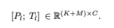
Hence instruction knowledge learned within Pl can effectively guide Tl to generate contextual responses.

The above image shows that all N layers of the transformer are “frozen” and only Adapter comprise of learnable tensors (L learnable tensors, one for each of the top L layer). Furthermore while the transformer has vanilla attention layers, LLaMa adapters uses zero-init attention and gating mechanisms.
6. LORA: LOW-RANK ADAPTATION OF LARGE LAN-
GUAGE MODELS
LoRA[14] injects trainable rank decomposition matrices into each layer of the Transformer architecture thereby reducing the number of trainable parameters for downstream tasks. The parameters of the original pre-trained transformer remains frozen. LoRA drives intuition from Aghajanyan et.al [16] which shows that the learned over-parametrized models in fact reside on a low intrinsic dimension. This led to the hypothesis that change in weights during model adaptation also has a low “intrinsic rank”,
The paper further states that LoRA allows to train some dense layers in a neural
network indirectly by optimizing rank decomposition matrices of the dense layers’ change during
adaptation instead, while keeping the pre-trained weights frozen.
Low Rank Decomposition

In the above image a m x n weight W is decomposed into m x k matrix A and k x n matrix B. In linear algebra, the rank[16] of a matrix W is the dimension of the vector space generated by its columns. This corresponds to the maximal number of linearly independent columns of W. Over parametrized weight matrices can contain linearly dependent columns, hence they can be decomposed into product of smaller matrices.
One of the most popular method to perform low rank decomposition is Singular Value Decomposition[17].

For a m x n matrix M, SVD factorizes M into orthonormal matrices U and V. V* is the conjugate transpose of V.
Calculating the SVD consists of finding the eigenvalues and eigenvectors of MMT and MTM. The eigenvectors of MTM make up the columns of V , the eigenvectors of MMT make up the columns of U. Also, the singular values in
LoRA’s LOW-RANK-PARAMETRIZED UPDATE MATRICES
For a pre-trained weight matrix W0 ∈ Rd×k LoRA constrains its update by representing the latter with a low-rank decomposition W0 + ∆W = W0 + BA, where B ∈ Rd×r, A ∈ Rr×k , the rank r min(d, k).

During training, W0 is frozen and does not receive gradient updates, while A and B contain trainable parameters.
Note both W0 and ∆W = BA are multiplied with the same input, and their respective output vectors are summed coordinate-wise. For h = W0x, our modified forward pass yields:
h = W0 x + ∆W x = W0 x + BA x
Random Gaussian initialization is used to initialize matrix A and matrix B is initialized to zero, so ∆W = BA is zero at the beginning of training.

For GPT-3 175B, the authors set a parameter budget of 18M (in FP16), that corresponds to r=8 if they adapt one type of attention matrix (from Query, Key and Value matrix) or r = 4 if they adapt two types of attention matrices for all 96 layers of GPT 3.
Adapting both Wq and Wv gives the best performance overall.
LoRA’s Effect On Inference Latency
Adding Adapter layers sequentially between Transformer’s layers induces inference time latency. There is no direct ways to bypass the extra compute in adapter layers. This seems like a non-issue since adapter layers are designed to have few parameters (sometimes <1% of the original model) by having a small bottleneck dimension, which limits the FLOPs they can add. However, large neural networks rely on hardware parallelism to keep the latency low, and adapter layers have to be processed sequentially. This makes a difference in the online inference setting where the batch size is typically as small as one.
When deployed in production, LoRA can explicitly compute and store W = W0 + BA and perform inference as usual. Note that both W0 and BA are in Rd×k . LoRA has no effect on inference time latency.
Finding The Optimal rank r for LoRA
Although LoRA already performs competitively for low values of r (4 and 8 in the above example), a natural question to ask is what’s the optimal value for r given a weight matrix W?
The authors in [14] check the overlap of the subspaces learned by different choices of r and by different random seeds. They showed that increasing r does not cover a more meaningful subspace, which suggests that a low-rank adaptation matrix is sufficient.
Grassmann Distance[19]
Grassmann distance helps us measure subspace overlap or similarity between the subspace spanned by column vectors of two matrices. Now given two low rank decomposition
Given low rank projection of weight matrix A into Ar=8 and Ar=64 which are the learned adaptation matrices with rank r = 8 and 64 using the same pre-trained model, [14] performs singular value decomposition and obtain the right-singular unitary matrices UAr=8 and UAr=64 . Then authors in [14]
ventured to answer the question, how much of the subspace spanned by the top i singular vectors in UAr=8 (for 1 ≤ i ≤ 8) is contained in the subspace spanned by top j singular vectors of UAr=64 (for 1 ≤ j ≤ 64).
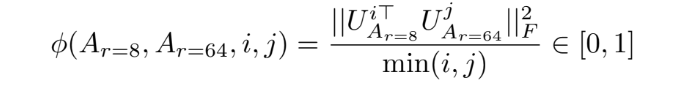
where Ui Ar=8 represents the columns of UAr=8 corresponding to the top-i singular vectors. φ(·) has a range of [0, 1], where 1 represents a complete overlap of subspaces and 0 a complete
separation. [14] shows that the top singular-vector directions of Ar=8 and Ar=64 are the most useful, while other directions potentially contain mostly random noises accumulated during training. Hence, the adaptation matrix can indeed have a very low rank.
7. Code Pointers
Colab link to fine tune quantized (int 8) 6B parameter Llama with LoRa
Download Llama in int 8 format
import os
os.environ["CUDA_VISIBLE_DEVICES"]="0"
import torch
import torch.nn as nn
import bitsandbytes as bnb
from transformers import AutoTokenizer, AutoConfig, AutoModelForCausalLM

model = AutoModelForCausalLM.from_pretrained(
    "facebook/opt-6.7b",
    load_in_8bit=True,
    device_map='auto',
)
tokenizer = AutoTokenizer.from_pretrained("facebook/opt-6.7b")
Freeze model parameters and cast Layer Normalization and head to FP16 for stability during training (original model is in int 8)
for param in model.parameters():
  param.requires_grad = False  # freeze the model - train adapters later
  if param.ndim == 1:
    # cast the small parameters (e.g. layernorm) to fp32 for stability
    param.data = param.data.to(torch.float32)

model.gradient_checkpointing_enable()  # reduce number of stored activations
model.enable_input_require_grads()

class CastOutputToFloat(nn.Sequential):
  def forward(self, x): return super().forward(x).to(torch.float32)
model.lm_head = CastOutputToFloat(model.lm_head)
Apply LoRA PEFT wrapper to 8 bit Llama
from peft import LoraConfig, get_peft_model

config = LoraConfig(
    r=16,
    lora_alpha=32,
    target_modules=["q_proj", "v_proj"],
    lora_dropout=0.05,
    bias="none",
    task_type="CAUSAL_LM"
)

model = get_peft_model(model, config)
print_trainable_parameters(model)
Here we are only adding adapters for Query and Value attention matrices. The rank parameter is 16.
The output shows that only .13% parameters of the 6.6 B parameter Llama model.
trainable params: 8388608 || all params: 6666862592 || trainable%: 0.12582542214183376
References
- Scaling Instruction-Finetuned Language Models
- LLaMA: Open and Efficient Foundation Language Models
- Alpaca: A Strong, Replicable Instruction-Following Model
- LLM-Adapters: An Adapter Family for Parameter-Efficient Fine-Tuning of Large Language Models
- https://www.nvidia.com/en-us/data-center/a100/
- Scaling Down to Scale Up: A Guide to Parameter-Efficient Fine-Tuning
- The Power of Scale for Parameter-Efficient Prompt Tuning
- Prefix-Tuning: Optimizing Continuous Prompts for Generation
- Parameter-Efficient Transfer Learning for NLP
- Parameter-efficient Multi-task Fine-tuning for Transformers via Shared Hypernetworks
- Query-Key Normalization for Transformers
- MetaWeighting: Learning to Weight Tasks in Multi-Task Learning
- LLaMA-Adapter: Efficient Fine-tuning of Language Models with Zero-init Attention
- LoRA: Low-Rank Adaptation of Large Language Models
- Armen Aghajanyan, Luke Zettlemoyer, and Sonal Gupta. Intrinsic Dimensionality Explains the Effectiveness of Language Model Fine-Tuning. arXiv:2012.13255 [cs], December 2020.
- https://en.wikipedia.org/wiki/Rank_(linear_algebra)
- https://en.wikipedia.org/wiki/Singular_value_decomposition
- https://web.mit.edu/be.400/www/SVD/Singular_Value_Decomposition.htm
- https://en.wikipedia.org/wiki/Grassmannian
Posted in performance efficient fine tuning, Uncategorized
Tagged adapters, gpt, large language model, llama, lora, machine learning, nlp, peft
Leave a comment
Neural Ranking Architectures
Glimpses On Implicit/Explicit, Dense/Sparse, Gated/Non Gated, Low Rank And Many More Layered Interactions

101 Ranking Model Architecture
Neural ranking models are the most important component in multi stage retrieval and ranking pipeline. Whether it is e-commerce search, ads targeting, music search or browse feed ranking, ranking model will have the final say in selecting the most relevant entity for a given request. Improvement in ranking model’s architecture (as well as feature space) can have a direct impact on boosting the business KPI.
In this post I would discuss brief history of development around ranking model architectures. I woulds show how the core model architecture evolved with each major break-though in neural architecture development.
Part 1 — Genesis
In this section I would quickly go over some early model architectures and would discuss some key issues involved with them.
A. Issues With Wide Only Model

Wide only model (no representation learning) learns weights for individual features and their corresponding interactions. Key issue with this approach is that
- There is no generalization.
- We can’t learn interactions in absence/sparsity of training data
- Shallow Architecture — Single layer model, no feature transformation
B. Factorization Machine, Steffen Rendle, 2010
Given a real valued feature vector x ∈ Rn where n denotes the number of features, FM estimates the target by modeling all interactions between each pair of features
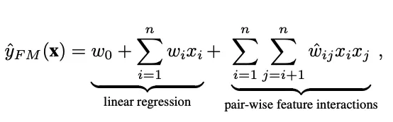
- w0 is the global bias
- wi denotes the weight of the i-th feature
- wij denotes the weight of the cross feature xi * xj
- (factorization) -> wij = vTi vj , where vi ∈ Rk denotes the embedding vector
In this architecture we project sparse features onto low dimensional dense vectors and learn feature interactions. Along with learning weights over individual sparse features (id based features, gender, categories etc), we learn their interactions via pair wise dot product of their representations.
Advantages of Factorization Machines
- Can generalize better
- Can handle sparsity w.r.t training data e.g. even if we have never seen interaction between Age 12 and Ad Category Gaming in training data, at inference time we can learn their interaction value by using corresponding embedding’s dot product
Disadvantages of Factorization Machines
- Shallow Structure — Limited Capacity Model (low representation power)
- Lacks feature transform capability
- Lacks ability to use embeddings based features (we can’t use pretrained embeddings for a feature)
C. Wide & Deep — Poor Man’s Ranking Model

This architecture has two key components, a wide part (dealing with float value and binary features) and a deep part (learns representations of sparse id based features). Wide part focuses on memorization and deep part on generalization. By jointly training a wide linear model (for memorization) alongside a deep neural network (for generalization), one can combine the strengths of both.
Wide Network
- Manually created handcrafted interaction features
- Helps in “Memorization” of important interactions
- No Dense Sparse Interaction — Sparse (embedding) features interact in deep part of the network but they don’t interact with the dense part of the network
- No transformations for the dense feature layer
- Uses FTRL for optimization
Sparse Network
- Fully connected Network
- Uses different optimizer than wide part (AdaGrad)
- No explicit interactions : We have a fully connected network which created implicit interactions between features e.g. we can’t learn explicit interaction between category embedding and user embedding for an e-commerce product to learn user proclivity for that category.
D. Attention Factorization Machines
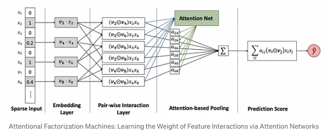
Like factorization machines, this method performs pair wise interactions between representations of features. But to improve over that method it uses attention based pooling mechanism to assign higher weights to most relevant interactions.
E. Deep & Cross — Deep & Cross Network For Ad Click Predictions
This architecture introduces the notion of “explicit” feature interactions.

Implicit Cross (think image representation) : Interaction is learned through end to end function without any explicit formula modeling such cross. The aim is to learn a high level representation e.g. a feature map in CNNs.
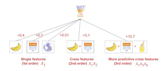
Explicit Cross (think gender * age * music genre interaction) : Modeled by an explicit formula with controllable interaction order. Aim is to learn weights over these explicit feature crosses.

Deep & Cross : Leverage implicit high-order crosses learned from DDNs, with explicit and bounded-degree feature crosses which have been found to be effective in linear models. One part of the network (left part) focuses on creating explicit feature crosses via a controllable function while the other part of the network (right part) is a deep network that learns implicit feature interactions.
Cross Network In Details
In the cross network we use following interaction formula

Here each layer would create interaction between output of previous layer and first layer (input layer), then we add the previous layer output as a residual skip connection. As we add more layers, we would generate higher order explicit interactions. We are learning previous layer’s interactions (layer L)via residual connection and adding more information to it via generating another higher order (L+1) interaction via taking element wise product of input vector with it.
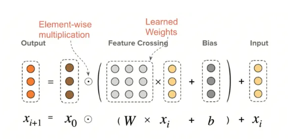
In the above image x0 is the input feature vector. x’ is output of last layer. x0 * x’ * w will perform a weight interaction . Weight matrix will learn which interactions are most important. First we will transform the xi layer (select most important crosses) and then interact it further with input vector to generate crosses of i+1 order.
Intuitive Explanation

In the above examples we have one user and one query feature in input vector (x0). Weight matrix is a binary matrix. The first order feature cross will generate user x query and query x user feature. As we add more layers we would have higher order features.
F: DCN V2 — DCN On Steroids
DCN V2: Improved Deep & Cross Network and Practical Lessons for Web-scale Learning to Rank Systems
With the aim to speed up learning and inference of DCN, the authors of DCN v2 introduces low rank factorization technique to cross feature computation. In DCN we were learning a weight matrix at each layer to transformer input of previous layer before performing Hadamard product with input vector. This process is computationally intensive.
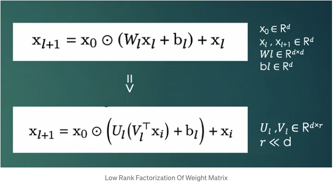
DCN V2 computes low rank factorization of the weight matrix and learns matrix U and V (in the above image) as part of training. This process drastically reduces number of parameters of the model and speeds up training as well as inference.

Part 2 Handcrafting Ranking Model Architecture
In this section we would take learning from part 1 and use them to create ranking model architecture.
A. Baseline Model

In this architecture we have try to divide the model layers into following components
- Input Layer — contains float value features, categorical id based features and embedding based features
- Feature interaction layer : this can be performed in various ways as discussed in earlier posts
- Transformations : Higher layers to transform the interacted features
Dense Features (float value features) transformation
In the baseline model we transform the dense features via a fully connected (FC) layer with non linearity to generate dense representations. The output of this layer is concatenated with feature interaction layer.
Sparse Feature Interactions
We can drive the intuition for this step from Factorization Machines discussed in Part 1.B
In this layer we take pair wise dot product of embeddings of all sparse (id based ) features e.g. user embedding * product embedding, user embedding * brand embedding etc.
After concatenating the output of the above two steps we further transform them to learn generalized representation. Finally a sigmoid unit decides the click probability.
B. Dense Sparse Interactions
In the last architecture we performed sparse feature interactions but skipped dense — sparse interactions. Dense features contain bias information e.g. age, gender of user, price of product, popularity score, trending score etc. of the product. When interacted with sparse features, we can gain valuable higher order features. The idea for this type of interactions was first discussed in DeepFM: A Factorization-Machine based Neural Network for CTR Prediction

C. Dense Gating
As discussed in the above architecture, dense features have very critical information that acts like bias for the model. But given the context, important of different dense features can vary e.g. in Ad ranking model, if ads category is gaming then age of the user can be very relevant dense feature. To provide these features higher weight we will use Dense Gating mechanism.
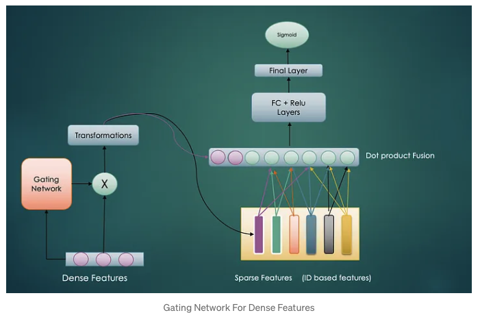
The gating network will learn to select the most important dense features and then transform them to generate dense representation. By introducing the dense gating mechanism, we can control the activation of each dense feature differently before we apply the shared weight matrix.
D. Memorization — Adding feature interaction output to final layer
Final layer is usually considered as an approach to memorize specific patterns for the model (in contrast, deep neural network before the final layer is more about generalization power).

E. Further Optimization
We can perform many other optimizations to the above architecture e.g.
- Increase size of sparse embeddings
- Increase dense feature projection
- Increase Over Arch layer dimensions
- Increase Final layer dimensions
- Layer Normalization
- Position Weighted Features
- Attention Factorization Machines : uDifferent feature interaction might have different importance for the prediction task. (User gender = male) * (User watch history contains genre rock) might be more important than (User gender = male) * (Query Text Embedding)
Feature Fusion For The Uninitiated

Consider a typical e-commerce product. It would have a variety of content specific features like product title, brand, thumbnail etc and other engagement driven features like number of clicks, click through rate etc. Any machine learning model ingesting features of this product(e.g. product ranker, recommendation model etc.) would have to deal with the problem of merging these distinct features. Broadly speaking we can divide these features in following categories
- Dense Features
- Counter : #times clicked in k days/hours
- Ratio : CTR of entity
- Float: Price
- Sparse Features
- Category Id
- Listing id : [ids of last k products clicked]
- Rich Features
- Title Text Embedding
- Category/Attributes Embedding
In a Neural Network if we step beyond the input layer, a common problem faced is around fusing (merging) these features and creating a unified embedding of the entity (e-commerce product in our case). This unified embedding is then further transformed in higher layers of the network. Considering the variety of features (float value features, embedding based features, categorical features etc), performance of the model depends on when and how we process these features.
In rest of the post we would discuss various feature fusion techniques.
Embedding Feature Fusion Techniques
For the sake of simplicity we would first consider the case of how to handle multiple embeddings in the input feature layer. Later on we would include architectural techniques to merge dense (float value features). As an example if we are building a music recommendation model, one of the input to the recommender may be embeddings of last k songs listened by the user or embeddings of genres of last k songs listened. Now we would want to fuse(merge) these embeddings to generate a single representation for this feature. Next section would discuss techniques to combine these embeddings in the input layer and generate a unified embedding.
Method 1 – Concatenate And Transform
In the diagram below, input layer can have text, images and other types of features. Respective encoder would process the corresponding input (e.g. pre-trained Resnet can generate image embedding, pre trained BERT can generate text embedding etc) and generate an embedding. These embeddings are represented as vector-1, vector-2 and vector-3.
In concatenation based fusion technique we would concatenate embeddings belonging to each modality and then pass it through a fully connected network.

Method 2 – Pooling
Another light weight technique is use techniques like mean and max pooling. In the image below, Youtube session recommender is fusing embeddings of watched videos in a session using average of their embeddings.

Method 3 – Pair Wise Dot Product
In this method we would take pairwise dot product of each embedding (vectors in the image below). After the pair wise dot products we would further use MLP (or Full connected) layers to transform it.


One of the drawback of this technique is its computational complexity. Due to quadratic computational complexity, the number of dot products grow quadratically in terms of the number of embedding vectors. With increasingly input layer, the connection of dot products with fully connected layer can become an efficiency bottleneck and can constrain model capacity.
To overcome this issue we can resort to Compressed Dot Product Architecture discussed in the next section
Method 4 – Compressed Dot Product Architecture

In the above figure we have showcased pairwise dot product fusion as matrix multiplication. Consider X as a matrix of feature embeddings. Here we have 100 features and each feature embedding is of length 64. Pair wise dot product can be view as a product of feature matrix and its transform.
The compression technique exploits the fact that the dot product matrix XXT has rank d when d <= n, where d is the dimensionality of embedding vectors and n is the number of features.
Thus, XXT is a low rank matrix that has O(n*d) degree of freedom rather than O(n2). In other words, XXT is compressible. This is true for many current model types that have sparse input data. This allows compression of the dot product without loss of information.

- X is an n*d matrix of n d-dimensional embedding vectors (n=100;d=64).
- Per techniques described herein, instead of calculating flatten(XXT), flatten(XXTY) is calculated.
- Y is an n*k matrix (in the example k=15).
- Y is a learnable parameter and is initialized randomly.
XXT would lead to n * d * n operations, where as dot product compression XXTY would take O(n * d * k) operations (k is very less than n).
Y is a learnable parameter and is initialized randomly. Y can be learnt, alongside other parts of the model. The projection through Y significantly reduces the number of neurons passing to the next layer while still preserving the information of original dot product matrix by exploiting the low rank property of the dot product matrix.
One of the drawback of this approach is that learned matrix Y becomes independent of the input. It would have same values for all inputs. To resolve this issue, we can use attention aware compression (please refer to Dot Product Matrix Compression for Machine Learning for more details).
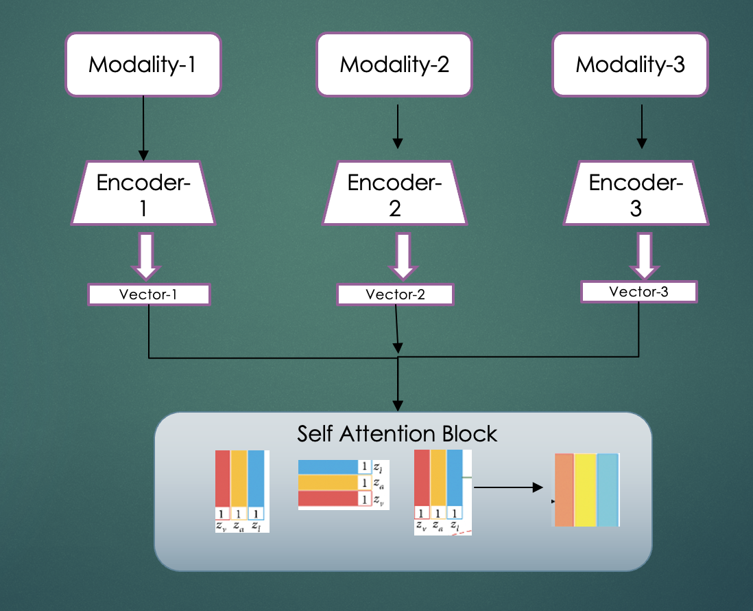
Method 5 – Attention Fusion
In this approach we follow the self attention logic to fuse different embeddings.
Method 6 – Tree based Fusion
In this technique we concatenate the feature embeddings and provide them as a single input to a Tree Ensemble Model e.g. Boosted Trees or GBT. This model will be separately trained from the main neural network. In this phase we would take output of leaves of each tree in the ensemble. In the image below these are depicted as h1, h2 etc. The fused (transformed) embedding will be concatenation of the output of leaves (h1 + h2 + ..). This will be provided as input to the main neural network. On a high level this acts as a non linear transform of input features.

Dense (Float) Features Fusion
The special case for feature fusion is for float value features. Unlike embedding based feature fusion, here we have just one vector of float features (e.g product price, click through rate, add to cart rate etc.). For handling dense features we would pass them through a fully connected layer with non linearity. This will lead to a transformed representation that would either concatenated or interacted with sparse fused features.

Baseline Model
An example architecture for a baseline model is described below

In this architecture we are first performing fusion of dense features. Separately sparse features (or embedding features) will have dot product fusion in a separate layer. As next step we are concatenating the fused vector of dense and sparse vectors in the interaction arch. In the next part of the network we are performing transformations over the concatenated feature vector.
Dense Sparse Feature Fusion
The last piece of the puzzle is how to interact the dense features and sparse features. Till now we have seen embedding based feature fusion (let’s say via dot product fusion) and dense (float value features) fusion. In this section we would explore how to interact (fuse) them together.

For dense-sparse interactions we would first generate an intermediate representation of the dense features via performing a non linear transform. Then we would perform following two steps
- Concatenating transformed dense feature representation to interaction layer
- Stacking the transformed dense feature representation with embedding inputs
In this way the dense transformed representation (output of FC + Relu layer) would take part in dot product fusion, hence it will interact with the individual embeddings of the input layer. Since dense features contain bias information (e.g. CTR or number of clicks provide bias about product performance), we would want to preserve this information. Hence in a residual connection kind of way we concatenate the transformed dense representation with the output of dot product fusion.
Posted in Uncategorized
2 Comments
Graph Neural Networks Based Attribute Discovery For E-Commerce Taxonomy Expansion
Previous post on Attribute Discovery
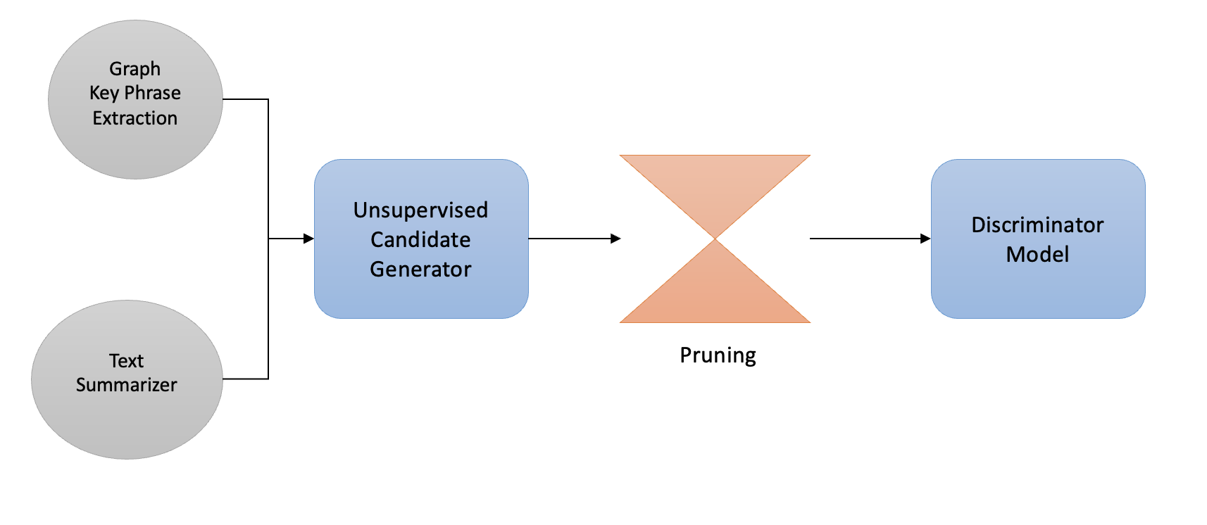
In Part 1 of Attribute Discovery we discussed unsupervised approaches that used Graph based Keyword and Key Phrase extraction algorithms to generate a list of candidate tokens that can be potential attributes missing from e-commerce taxonomy. We furthermore talked about various heuristics like statistical pruning and syntactic pruning based filtering techniques. This article goes one step further to dig into supervised modeling based methods to further remove noisy candidates.
As discussed in the last part of this series, one of the foremost drawback of using a totally unsupervised method for keyword extraction is that we don’t learn from our mistakes once we get feedback on extracted keywords from a Taxonomist or a human labeler. Another issue is that without a model based approach for keyword extraction, we miss out on using approaches like Active Learning that can guide us in creating better training data and hence a better feedback loop to get the contentious data points labeled. The unsupervised keyword extraction techniques are not domain sensitive i.e. they are not tunable to adapt to the data domain or topic and spits out lots of generic keywords that are not important for the domain under consideration. Also the share number of candidates generated are hard to get labeled, so we definitely need a mechanism to rank them in order of importance and get a feedback from domain experts.
Also we are not exploiting the information at hand i.e. attributes that are already part of the taxonomy. Take an example, if we already know that for category Clothing>Kids>Shoes, Color attribute type has values Green, Black And White in our Taxonomy; and candidate generator spits out new candidates as Brown and Blue, we should be able to use the data points already available to us (Green, Black and White) in associating the new keywords (Brown and Blue) to attribute type Color.
After extracting important keywords and candidate brand tokens, we would like to answer following questions
- Whether the new keywords belong to existing attribute types? — Attribute Type Detection
- If not can we group the keywords together so that similar keywords may belong to a new attribute type? — Attribute Type Discovery
To check whether a given keyword belong to a an existing attribute type we try link prediction[1] and node classification[2] based analysis using graph convolutional networks(GCN)[3].

Reference: https://tkipf.github.io/graph-convolutional-networks/
In message passing methodology, in each iteration every node gets messages from neighboring nodes and using their representations (messages) and it’s own representation, a new representation is generated. This involves application of aggregate functions and non linear transformations.

In the above figure node A will receive representations of neighboring nodes B, C and D and after applying linear transformations , permutation invariant aggregation operator (sum, average etc.) and applying further non linear transforms generates a new representation for node A.
These representations are further used for a downstream task like link prediction, node classification, graph classification etc.
Link Prediction[1]
Data :
- Keywords extracted from product title and description of products from Baby & Kids//Strollers & Accessories//Strollers
- Known Attribute Types and their corresponding values in category Baby & Kids//Strollers & Accessories//Strollers i.e. data from the Taxonomy
Heterogeneous Graph Creation
In this approach we first create a graph in which nodes are represented by the extracted keywords and links between them exists if and only if they occurred alongside each other in product title and description text more than a certain number of times. Furthermore we add extra nodes to the graph that represent attribute type e.g. Brand node, Stroller Type Node etc. Additional links were created between the nodes representing the attribute types and their synonyms from the rules table. To make graph dense we added a “pseudo(dummy)” node with category name “stroller”. This node will act as a context node and provide path between existing attribute value nodes (as well as attribute type nodes) and new attribute value candidate (keyword nodes)
Types of Edges
- Brand Node and known brand values
- Stroller Type Node and known stroller type values
- Dummy node “stroller” and keywords occurring in neighborhood of it in product titles and descriptions
- Candidate keywords and rest of nodes occurring in neighborhood of it in product titles and descriptions
Objective : Given two nodes if an edge exist between them. For our use case this would mean given an Attribute Type node e.g. Brand or Stroller Type, whether a link exist between them and candidate keyword.
Node Feature :
Each node has a 100 dimensional feature vector as an attribute. These vectors are word embeddings generated using Fasttext[5].
Category : Baby & Kids//Strollers & Accessories//Strollers

Train/Test Node Tuples
After creating the graph we split the links into train and test dataset. Positive examples include node tuples where edge exists in the graph and for negative examples we created synthetic hard negative examples e.g. tuples created from sample from brand nodes and stroller type attribute values.
Model Architecture

We used Tensorflow based Stellar Graph[4] for creating a 2 GCN layer network with the last layer as binary classification layer. The hidden layer representations of both inout nodes are aggregated using point wise product and the final “edge” representation is forwarded to the binary classification layer. Adam optimizer was used to calculate gradients for back propagation.
Input : word embeddings of tuple of nodes representing an edge e.g. if an edge e is formed by vertices “Brand” and “graco” then word embedding of these two nodes would be input to the node.
Link Prediction Results
The plots below shows the link prediction probabilities on test and train data set.


Attribute Type Prediction And Issues
In the last phase we input node ids for new extracted keywords and Stroller Type attribute node to check if a link exists between them. Similarly we input brand candidates and Brand node id tuples to check if a link exists between the Brand node and new brand candidates. The results of this experiment were really bad as it seems the model is overfitted. Also there is a semantic issue with the links in the graph. One half of edges represent keyword proximity in product title and description whereas other links represent connection between attribute type and synonyms. This discrepancy in the meaning of edges in the graph may be casing issues with low link prediction accuracy on the new data set.
Node Classification[2]
In this second experiment we intend to classify the nodes in the keyword graph to its corresponding attribute type. In this graph each node has an optional attribute representing the class of the node e.g. Brand or other Attribute Type. Graph is formed based on keyword proximity in product title and description text. No additional attribute type nodes are added to the graph like we did in previous link prediction task.
Data:
Category : Toys & Games//Remote Control Toys//Cars & Trucks
- Data Instances : ~16k product titles and descriptions
- Attribute Values and Attribute Types in the Taxonomy for category Cars & Trucks
- as class of the attribute values
Node Features
Each node is represented by 50 dim word embedding generated from Fasttext and 5 dim embedding generated by poincare embeddings from the keyword graph. Poincare embeddings will contain the hierarchical (positional) details of the node in the graph.
Homogeneous Graph Creation
In this graph each node has an optional attribute representing the class of the node e.g. Brand or other Attribute Type. Graph is formed based on keyword proximity in product title and description text. No additional attribute type nodes are added to the graph like we did in previous link prediction task.
Like the earlier experiment we added additional nodes representing known attribute values e.g. known brands and vehicle type etc. To make the graph sufficiently dense, we again added dummy nodes for “car” snd “truck” (tokens in category name). Edges exist only when two tokens occur together in product title or description.

Model Architecture

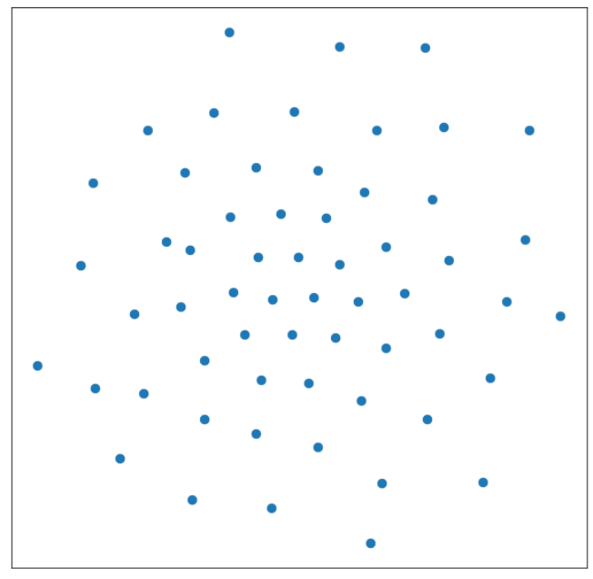
Visual Analysis
To get visual intuition around effect of training on node representations, we would compare 2D TSNE representations of node feature embeddings before and after training.
Before Training : Train Node Feature Projection In 2D using TSNE

After Training : Train Node Feature Projection In 2D using TSNE

We generate the node representations by feeding the network feature vector of the node (fasttext word embedding concatenated with node’s poincare embedding) and generate the representation from the second GCN layer. (second hidden layer) We can clearly see that in 2D nodes belonging to same attribute type are closer to each other after training the network.
Testing the trained mode on new extracted keywords
In a similar fashion we generate the representation of the newly extracted keywords. The plots below show low dimensional visualization using TSNE of original feature vector of the extracted keywords vs representations generated from trained network.
Plot original feature vectors of keywords with unknown attribute type ( TSNE)
There seems to be no apparent structure in the above plot.
Plot GCN transformed representations of keywords with unknown attribute type (TSNE)

The above plot shows 2 clusters in data, one near the origin and second on the other side of the diagonal.
Node Classification Results
We had 59 keywords where we are unaware of the attribute types.
Threshold Creation
In this step we run the training data through our network and get the max predicted probabilities ie for each node where attribute type is known, classify it using the trained model and select the maximum from the softmax layer.
After that find the 90th percentile from list of output probabilities in the last step. This would be used as classification threshold on data where attribute types are unknown.

Node classification maximum class probability on training data
In the last step the extracted keywords are fed into the network and maximum of softmax layer is compared with the threshold compared in last step. Only when the predicted probability is greater than the calculated threshold than only we would consider the predicted class.
Output :
keyword: run, predicted attribute type: brand
keyword: jeremy, predicted attribute type: rc scale
Both seems to be misclassification.
Hierarchical Clustering the transformed representations of new keywords
After training the model on all the labeled nodes we generated representation of all nodes where class is not available i.e. nodes where we don’t know the attribute type. After that we perform hierarchical clustering on these representations.

It seems three clusters exist in our data. The contents of the clusters are as follows
Cluster 1 = ['kit', 'scale', 'bodied', 'diecast', 'toy', 'red', 'redcat',
        'jeremy', 'mayfield']
Cluster 2 =  ['rc', 'nitro', 'work', 'model', 'brand', 'custom', 'light', 'rear',
        'seat', 'speed', 'ship', 'ford', 'barbie', 'power', 'like', 'race',
        'pickup', 'condit', 'baja', 'vxl', 'talion', 'partes', 'black',
        'lamborghini', 'look', 'spiderman', 'indy', 'conteol', 'lowrider']

Cluster 3 = ['charger', 'good', 'need', 'box', 'control', 'vw', 'batterie',
        'come', 'remot', 'price', 'wheel', 'ride', 'drive', 'atv', 'kid',
        'jeep', 'run', 'include', 'tire', 'upgrade', 'motor']
The intuition behind this experiment was that after GCN transformations newly discovered keywords that are similar to each other would group together in one cluster and that cluster may be represented by an attribute type.
Conclusion
We discussed various approaches that don’t solve the problem of attribute extraction individually but as a whole, pipeline comprising of the above steps as individual component can provide us an unsupervised way to generate candidate attribute values and brands that can be further pruned by taxonomists. This approach can save us lot of time by automating the attribute discovery phase and providing not only important keywords/brands but also synonyms present in data that can be further used to increase coverage. The proposed tool is neatly laying down all the relevant information about about every category that the taxonomist needs in form of keywords, brands and attributes.
References
Posted in Uncategorized
Leave a comment
Attribute Discovery For E-Commerce Taxonomy Expansion – Part 1 Unsupervised Graph Based Keyword Extraction

During my time at Facebook Marketplace I worked at a very esoteric problem of semi automating attribute discovery i.e. finding granular attribute values from product titles and description that are not present in the Product Attribute Taxonomy. Each category in e-commerce catalog has a unique set of attribute types and values e.g. Clothing > Men’s > Shirt can have Colors, Size, Pattern, Brand Attribute Types and each attribute type will have given set of values (Size can X, S, M, L, XL etc). These attributes play critical role in Query Understanding Models as well as act as critical features in Retrieval and Ranking Models. So the richer the Attribute Taxonomy is, the better would be customer experience.
At most of the e-commerce companies the current process to find these attributes involves manual analysis of data and other data sets by Taxonomists. The existing approach is a top down approach i.e. for each category Taxonomists would do competitor analysis and create attribute types and their corresponding values relevant to the concerned category.
Some of the drawbacks of manual attribute creation are
- Scalability issues : Hard to keep up with creation of attribute types and values with more and more products/catalog being added to the catalog
- Low Coverage : There is no way to discover attribute values present in out data that corresponds to an attribute type. This often leads to low coverage.
- Rules/Synonyms creation : synonyms for attribute values are manually curated and in the existing pipeline coverage is directly proportional to quantity of synonyms an attribute value has.
The rest of the document would discuss some approaches that can be used to automatically discover attribute values and group similar attribute values that may represent potential attribute type. Furthermore we would try to extract all relevant synonyms for the discovered attributes. This approach is a bottom up approach i.e. we would look at the data first and then come up with a set of attributes.
Attribute Discovery Process
The proposed attribute discovery approach is unsupervised in nature. The procedure broadly involves hierarchical clustering the data and extracting relevant keywords from each cluster. In the next step we would try to further prune and cluster the keywords that are similar to each other. The aim of the proposed approach is to present clusters of high quality keywords from different categories to the taxonomists and thereby save their time and effort. By highly quality we mean keywords that are not only statistically relevant but also define either some property or quality of the core entity described in the category e.g. for category Baby & Kids > Diapering > Cloth Diapers we would want to automatically create a list of following keywords [small, large, prefold, resusable, snap, pocket, inserts, covers, lot, size, liner, organic, bamboo] that defines the properties of diapers and a second list that may contain probable brands associated with clothing diapers e.g. Bumgenius, Thirsties, Grovia, Alva, Panales, Tela. In the final step a Taxonomist can prune or select the proposed keywords.
PART 1 Analysis
Step 1: Product Representation Creation
For the experimentations sake we have only considered product title and description features to create product representation. We used pre trained Hugging Face sentence transformer to generate product embeddings of length 768. Although better representations can be created that can use other product features like image, prices etc.
Step 2: Hierarchical Clustering
In this step we performed Ward Hierarchical Clustering[1] on the 905 X 768 matrix created in the last step.

The above dendrogram plot indicates that there are 4 clusters in the Clothing Diapers Category. In Semi-supervized Class Discovery [2] and PinnerSage: Multi Modal User Embedding Framework For Recommendations[3], researchers at Google and Pinterest respectively have used similar kind of hierarchical clustering approaches to club similar products for further analysis.
Later on we would want to automate the process of detection of optimal numbers of clusters.
A quick look at the word clouds of 1st and 2nd cluster provides a glimpse into different prominent keywords present the corresponding clusters.

Cluster 1

Cluster 2
Step 3: TextRank: Keyword Extraction
This step involves extracting most relevant keywords from the clusters created in last step. We use TextRank[4], a graph based ranking model for text processing. TextRank creates a graph from tokens presents in product titles and descriptions, after certain preprocessing it uses a scoring model to rank nodes in the graph. TextRank[4] provides better results from statistical and lexical analysis based approaches. We tried exploring other methods like EmbedRank[5], that uses embedding based similarity between sentences and the whole corpora but found that TextRank best suits to our use case.
List of most relevant keywords from first cluster (applying stemming and grouping similar tokens)
('insert', ['insert', 'inserts', 'inserted']),
 ('size', ['size', 'sized', 'sizes']),
 ('cover', ['covers', 'cover']),
 ('brand', ['brand', 'brands']),
 ('lot', ['lot', 'lots']),
 ('newborn', ['newborn', 'newborns']),
 ('pocket', ['pocket', 'pockets']),
 ('small', ['small']),
 ('new', ['new']),
 ('prefold', ['prefolds', 'prefold']),
 ('snap', ['snaps', 'snap']),
 ('bag', ['bag', 'bags']),
 ('bumgenius', ['bumgenius']),
 ('thirsties', ['thirsties']),
 ('liner', ['liners', 'liner']),
 ('included', ['including', 'includes', 'included']),
 ('bum', ['bum', 'bums']),
 ('bamboo', ['bamboo']),
 ('white', ['white']),
 ('reusable', ['reusable']),
 ('organic', ['organic']),
 ('velcro', ['velcro']),
 ('lbs', ['lbs']),
 ('large', ['large'])
The above mapping provides us a candidate list of attribute values and their corresponding synonyms.
Step 4: Semantic Association Between Important Keywords : Network Based Analysis
After creating an initial list of candidate attribute values, the intuitive next step would be to group so that each group can be defined by an attribute type and further prune the candidate list to get most relevant keywords pertaining to category “Cloth Diapers”.
Example: In the above list “pocket”, “prefold”, “snap”, “size” defines properties of cloth diapers but “velcro” is a property of “pocket”.
In this step we create a graph of tokens extracted in last step based on their proximity in the product titles and descriptions. In this experiment we create an edge between nodes only if the corresponding keywords are within a window size of 1 i.e. adjacent to each other. We use python networx[6] for creating a directed acyclic graph(DAG) of keywords.

The above DAG clearly shows some interesting properties of our attributes.
- The red colored edges show direct associations of “cloth diapers” i.e. core attributes of cloth diapers.
- Connection between Velcro node and Pocket node shows that velcro is an aspect of pocked diapers.
- Similarly color “white” is an attribute of “liner” and “velcro” nodes.
- Two directed edges between Brand and Thirsties creates string association between them implying that Thirsties is a brand.
In similar manner we can make more inferences.
Step 5: Hierarchical Embeddings: Creating Hierarchical Relations Between Nodes
Once we have a DAG of important keywords and a natural next step would be to understand the hierarchy among the nodes. We would want to know the core nodes representing the backbone of the network and their associated satellite nodes.
Some of the ways that didn’t result into meaningful node associations
- PageRank: Apart from generating high ranking nodes, PageRank didn’t provide us any semantic information from the graph structure itself.
- Generating word embedding using FastText[7] and further using embeddings of the extracted keywords for hierarchical clustering.
In this step we generated POINCARE EMBEDDINGS[8] of the nodes of the graph created in last step.
 "Poincaré embeddings are a method to learn vector representations of nodes in a graph. The input data is of the form of a list of relations (edges) between nodes, and the model tries to learn representations such that the vectors for the nodes accurately represent the distances between them. The learnt embeddings capture notions of both hierarchy and similarity - similarity by placing connected nodes close to each other and unconnected nodes far from each other; hierarchy by placing nodes lower in the hierarchy farther from the origin, i.e. with higher norms.
The main innovation here is that these embeddings are learnt in hyperbolic space, as opposed to the commonly used Euclidean space. The reason behind this is that hyperbolic space is more suitable for capturing any hierarchical information inherently present in the graph. Embedding nodes into a Euclidean space while preserving the distance between the nodes usually requires a very high number of dimensions."[9]

We generated 2 D representations of the nodes using gensim.models.poincare[10]. The nodes near to the origin represents the root nodes of the graph. Node “clothing diaper” is at coordinate 0,0. thereby suggesting that it is the root node (key topic) of the graph. Nodes at the periphery like lbs, bum, new etc. are the leaf node and much down in the hierarchy i.e. not directly relevant to the root node “cloth diaper”.
To fetch the key attributes of clothing diapers we extract the nearest neighbors of the root node. The list below shows nearest neighbors with their corresponding
[('cloth diaper', 0.0),
 ('small', 0.1365535033774657),
 ('large', 0.17949012971429448),
 ('prefolds', 0.20087067143255224),
 ('reusable', 0.22612112692088746),
 ('inserts', 0.29712060251440736),
 ('bumgenius', 0.30584862418124015),
 ('covers', 0.3563740496401796),
 ('lot', 0.3919719432521571),
 ('pocket', 0.409106234142296),
 ('size', 0.4996583982212509),
 ('liner', 0.621093919540953),
 ('snap', 0.7515983205641947),
 ('organic', 0.8492109718887274),
 ('bamboo', 0.851353947350201)]
The above list shows some high quality candidates for attribute values associated with cloth diapers.
Step 6: Key Phrase Extraction And Text Summarization
Till now we have tried to extract important keywords descriptive of “clothing diapers” category. Another highly effective way to get a good idea of the context and use of different keywords w.r.t “clothing diapers” in all the product titles and descriptions is by text summarization. We used Spacy pytextrank[11] that creates a graph similar to keyword TextRank graph created in step 3 but uses phrases instead of keywords as graph nodes.
Summarization tries to paint a complete picture of the different topics discussed in the text. In our case the list below consists of all attributes and brands present in the clothing diaper category.
The tokens marked in bold represents probable brand names.

Part 2 – Multi Stage Approach : Brand Extraction
The first phase would generate a broad list of keywords using an ensemble of unsupervised methods. As we have seen earlier that output of keyword extraction algorithms is often noisy as well as contain generic keywords like “price”, “shipping”, “FCFS” etc. that are not category specific. Once a candidate set is generated we would like to apply a set of rules like blacklist keywords, noun/ pronoun detection, named entity detection and other heuristics to prune candidate list. Ideally a classification model should further classify the pruned set of candidates into probable attribute value or not. We would discuss this discriminator based methods in next part of this blog series.

Rest of the document would deal with explanation of the individual component described in the above architecture.
The proposed architecture comprise of two key components
I. Candidate Generation

From the plethora of approaches discussed in [12] and [13], the best methods of unsupervised keyword extraction are graph based. In step 6 (Keyword Extraction And Text Summarization) we have already seen that although the results of TextRank comprised of noise and generic keywords, the recall of category specific keywords was high.
In the first phase we can just run some out of shelf keyword extraction algorithms like the one discussed below and take a union of keywords set generated by them.
A. Graph Based Keyword Extraction Methods
Majority of the popular unsupervised approaches use graph based centrality measures like Eigenvector centrality and PageRank to find relevant keywords from co-occurence token graph of concerned text. Complex Network based Supervised Keyword Extractor[23] shows that although various centrality based metrics effectively captures node importance, however probability density distribution of strength for keywords and non-keywords for the training set prepared during their study shows overlapping areas near high strength values. The overlap indicates that strength alone is not an accurate discriminator between keywords and non-keywords. The experimental results of [23] validates our findings of extracting large number of false positive keywords when we used unsupervised methods like TextRank that uses PageRank bases graph centrality metric.
Graph Centrality Metrics
- Eigenvector Centrality : It quantifies a node’s embedded-ness in the network while recursively taking into account the prestige of its neighbors.
- PageRank : It computes the prestige of a node in the context of random walk model.
- PositionRank: An extension of PageRank that is based on the intuition that keywords are likely to occur towards the beginning of the text rather than towards the end.
- Coreness: Coreness is a network degeneracy property that decomposes network G into a set of maximal connected subgraphs, such that nodes in each subgraph have degree at least k within the subgraph. Coreness of a node is the highest core to which it belongs.
- Clustering Coefficient : Clustering coefficient of a node indicates edge density in its neighborhood. It is a local property.
- Strength of a node : Strength(weighted degrees) of a node measures its embedded-ness at local level.

Graph Based Keyword And Key Phrase Extraction Algorithms
- TextRank[4]
- Only use nouns and adjectives as nodes in the graph
- no edge weights for keyword graph
- SingleRank[14]
- incorporates weights to edges, the co-occurrence statistics are crucial information regarding the contexts
- RAKE [15] (Rapid Automatic Keyword Extraction)
- that utilizes both word frequency and word degree to assign scores to phrases
- SGRank [16] and PositionRank [17]
- stage 1
- utilize statistical, positional, and word co-occurrence information
- considers only noun, adjective or verb
- takes into account term frequency conditions
- stage 2
- the candidate n-grams are ranked based on a modified version of TfIdf
- stage 3
- the top ranking candidates are re-ranked based on additional statistical heuristics, such as position of first occurrence and term length
- stage 4
- the ranking produced in stage three is incorporated into a graph-based algorithm which produces the final ranking of keyphrase candidates
- stage 1
B. Topic Based Methods
- TopicRank [18]
- preprocesses the text to extract the candidate phrases. Then, the candidate phrases are grouped into separate topics using hierarchical agglomerative clustering
- In the next stage, a graph of topics is constructed whose edges are weighted based on a measure that considers phrases’ offset positions in the text.
- TextRank is used to rank the topics and one keyphrase candidate is selected from each of the N most important topics
- Salience Rank [19]
- It runs only once PageRank, incorporating in it a word metric called word salience Sα (w), which is a linear combination of the topic specificity and corpus specificity of a word (the last can be calculated counting word frequencies in a specific corpus). Intuitively, topic specificity measures how much a word is shared across topics (the less the word is shared across topics, the higher its topic specificity)
C. Graph-based Methods with Semantics
“The main problems of the topic-based methods are that the topics are too general and vague. In addition, the co-occurrence-based methods suffer from information loss, i.e., if two words never co-occur within a window size in a document, there will be no edges to connect them in the corresponding graph-of-words even though they are semantically related, whereas the statistics-based methods suffer from information overload, i.e., the real meanings of words in the document may be overwhelmed by the large amount of external texts used for the computation of statistical information.”[13]
Method 1 – Distant supervision using knowledge graphs[20]:
a. Nouns and named entities (keyterms) are selected and grouped based on semantic similarity by applying clustering
b. The keyterms of each cluster are connected to entities of DBpedia
c. For each cluster, the relations between the keyterms are detected by extracting the h-hop keyterm graph from the knowledge graph, i.e., the subgraph of DBpedia that includes all paths of length no longer than h between two different nodes of the cluster.
d. Then, all the extracted keyterm graphs of the clusters are integrated into one and a Personalized PageRank (PPR)[6] is applied on it to get the ranking score of each keyterm.
Method 2: WikiRank[21] is an unsupervised automatic keyphrase extraction method that tries to link semantic meaning to text
a. Use TAGME[8], which is a tool for topic/concept annotation that detects meaningful text phrases and matches them to a relevant Wikipedia page
b. Extract noun groups whose pattern is zero or more adjectives followed by one or more nouns as candidate keyphrases
c. A semantic graph is built whose vertices are the union of the concept set and the candidate keyphrase set. In case the candidate keyphrase contains a concept according to the annotation of TAGME an edge is added between the corresponding nodes
d. The weight of a concept is equal to the frequency of the concept in the full-text document.
e. The score of a concept c in a subgraph of G to be
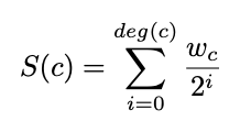
II. Candidate Pruning

Generic Keywords Filtering
The rule set would comprise of blacklist of keywords that are generic and doesn’t corresponds to any specific characteristic of product category. We can keep a global as well as category specific keyword list. Example keyword blacklist
keyword_blacklist = ["hola", "pick", "pickup", "cash", "collect", "locate", "work", "contact", "use", "locat", "news", "good", "total", "valu", "complete", "list", "sold", "know", "limit", "want", "complete", "near", "offer", "new", "date", "nice", "day", "interest", "ship", "sell", "item", "price", "need", "need", "link", "like", "sale", "includ", "free", "look", "condit", "ship", "www", "need", "great", "machine", "come", "sale", "item", "sell", "ask", "com", "like", "avail", "beauti", "excel", "look", "best", "thank", "meet", "came", "help", "got"]
Apart from creating a blacklist we can also use statistical analysis to study the spread/dispersion of a keyword across categories. A keyword with low inverse document score or coverage across categories should be automatically filtered.
Another set of rules would be extraction rules that would help us extract brands. These rule set would involve simple pattern matching components that would help us create a weak supervision system on the lines of how SNORKEL[22] works.
For brand extraction we perform following steps and then apply the following set of weak supervision rules
Heuristics Based Filtering
- Filter output candidates based on POS Tagging and NER Tagger output
- is candidate noun or pronoun
- is NER label ORG
- is first character upper
- Statistical Pruning
- is length less than 20 and greater than 3
- Filter candidates based on block word list
- Filter candidates based on dictionary check
- Filter Candidates based on syntactic check
- is candidate ASCII
- is not all numeric
- is not in english dictionary
One of the foremost drawback of using a totally unsupervised method for keyword extraction is that we don’t learn from our mistakes once we get feedback on extracted keywords from a Taxonomist. Another issue is that without a model based approach for keyword extraction, we miss out on using approaches like Active Learning that can guide us in creating better training data and hence a better feedback loop to get the contentious data points labeled. The unsupervised keyword extraction techniques are not domain sensitive i.e. they are not tunable to adapt to the data domain or topic and spits out lots of generic keywords that are not important for the domain under consideration. Also the share number of candidates generated are hard to get labeled, so we definitely need a mechanism to rank them in order of importance and get a feedback from domain experts.
Next post discusses semi supervised approaches to improve the attribute extraction process using Graph Neural Networks.
References:
- Ward’s Hierarchical Clustering Method: Clustering Criterion and Agglomerative Algorithm
- Semi-Supervised Class Discovery
- PinnerSage: Multi-Modal User Embedding Framework for Recommendations at Pinterest
- TextRank: Bringing Order into Texts
- Simple Unsupervised Keyphrase Extraction using Sentence Embeddings
- NetworkX: Network Analysis in Python
- Enriching Word Vectors with Subword Information
- Poincaré Embeddings for Learning Hierarchical Representations
- https://rare-technologies.com/implementing-poincare-embeddings
- https://radimrehurek.com/gensim/models/poincare.html
- https://spacy.io/universe/project/spacy-pytextrank
- A Review of Keyphrase Extraction
- Kazi Saidul Hasan and Vincent Ng, Automatic Keyphrase Extraction: A Survey of the State of the Art, Proceedings of the 52nd Annual Meeting of the Association for Computational Linguistics
- Wan, X. and Xiao, J. (2008) Single document keyphrase extraction using neighborhood knowledge. In Proceedings of the 23rd AAAI Conference on Artificial Intelligence, AAAI 2008, Chicago, Illinois, USA, July 13-17, 2008, 855–860. URL: http://www. aaai.org/Library/AAAI/2008/aaai08-136.php.
- Rose, S., Engel, D., Cramer, N. and Cowley, W. (2010) Automatic keyword extraction from individual documents. Text Mining: Applications and Theory, 1–20. URL: http://dx.doi.org/10.1002/9780470689646.ch1.
- Danesh, S., Sumner, T. and Martin, J. H. (2015) Sgrank: Combining statistical and graphical methods to improve the state of the art in unsupervised keyphrase extraction. In Proceedings of the Fourth Joint Conference on Lexical and Computational Semantics, Denver, Colorado, USA., June 4-5, 2015, 117–126. URL: http://aclweb.org/anthology/S/S15/S15-1013.pdf.
- Florescu, C. and Caragea, C. (2017b) PositionRank: An unsupervised approach to keyphrase extraction from scholarly documents. In Proceedings of the 55th Annual Meeting of the Association for Computational Linguistics, ACL 2017, Vancouver, Canada, July 30 – August 4, 2017, Volume 1: Long Papers, 1105–1115. URL: https://doi.org/10.18653/v1/P17-1102.
- Bougouin, A., Boudin, F. and Daille, B. (2013) TopicRank: Graph-based topic ranking for keyphrase extraction. In Proceedings of the 6th International Joint Conference on Natural Language Processing, IJCNLP 2013, Nagoya, Japan, October 14-18, 2013, 543–551. URL: http://aclweb.org/anthology/I/I13/I13-1062.pdf.
- Teneva, N. and Cheng, W. (2017) Salience rank: Efficient keyphrase extraction with topic modeling. In Proceedings of the 55th Annual Meeting of the Association for Computational Linguistics, ACL 2017, Vancouver, Canada, July 30 – August 4, Volume 2: Short Papers, 530–535. URL: https://doi.org/10.18653/v1/P17-2084.
- Shi, W., Zheng, W., Yu, J. X., Cheng, H. and Zou, L. (2017) Keyphrase extraction using knowledge graphs. Data Science and Engineering, 2, 275–288. URL: https://doi.org/10.1007/s41019-017-0055-z.
- Yu, Y. and Ng, V. (2018) Wikirank: Improving keyphrase extraction based on background knowledge. In Proceedings of the 11th edition of the Language Resources and Evaluation Conference, LREC 2018, 7-12 May 2018, Miyazaki (Japan), 3723–3727. URL: http://www.lrec-conf.org/proceedings/lrec2018/pdf/871.pdf.
- Snorkel: Rapid Training Data Creation with Weak Supervision
- Complex Network based Supervised Keyword Extractor
Posted in Uncategorized
1 Comment
