
Colab Link To Reproduce Experiment: LLM Compression Via Low Rank Decomposition.ipynb
Context
A neural network contains many dense layers which perform matrix multiplication. In the case of Transformers, Attention module has Key, Query, Value and Output matrices (along with the FF layer) that are have typically full rank. Li. et al. [3] and Aghajanyan et al.[4] shows that the learned over-parametrized models in fact reside in low intrinsic dimension. In popular Parameter Efficient Fine Tuning(PEFT) technique LoRA, the authors took inspiration from [3] and [4] to hypothesize that the change in weights during model adaptation also has a low intrinsic rank.
In real production models, the model capacity is often constrained by limited serving resources and strict latency requirements. It is often the case that we have to seek methods to reduce cost while
maintaining the accuracy. To tame inference time latency, low rank decomposition of weight matrices have earlier been used in applications like DCN V2[5].
Low Rank Decomposition
Low rank decomposition of a dense matrix 𝑀 ∈ R𝑑×𝑑 by two tall and skinny matrices
𝑈 ,𝑉 ∈ R𝑑×𝑟 helps us approximate M by only using U and V (way less parameters than original matrix M). Here r << d.

In the above image a m x n weight W is decomposed into m x k matrix A and k x n matrix B. In linear algebra, the rank[6] of a matrix W is the dimension of the vector space generated by its columns. This corresponds to the maximal number of linearly independent columns of W. Over parametrized weight matrices can contain linearly dependent columns, hence they can be decomposed into product of smaller matrices.
One of the most popular method to perform low rank decomposition is Singular Value Decomposition[7].
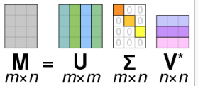
For a m x n matrix M, SVD factorizes M into orthonormal matrices U and V. V* is the conjugate transpose of V. 
Calculating the SVD consists of finding the eigenvalues and eigenvectors of MMT and MTM. The eigenvectors of MTM make up the columns of V , the eigenvectors of MMT make up the columns of U. Also, the singular values in
In this post I further explore effects of taking low rank decomposition of attention weight matrices (Query, Key, Value and Output) on T5-base performance.
Spectrum Decay
This section plots the Singular values of Query matrix of last decoder layer of flan-base (~220 million params) and flan-large (~700 million params) models.
Flan Base Weight Matrix (768 x 768)  = decoder.block[11].layer[0].SelfAttention.q.weight

Flan Large Weight Matrix (1024 x 1024) = decoder.block[23].layer[0].SelfAttention.q.weight
The above plot shows the singular value decay pattern of the learned weight matrices from flan-t5-base and flan-t5-large. The above plot shows a much faster spectrum decay pattern than a linear decline, reinforcing our hypothesis that Large Language Models have intrinsic low rank.

The above plot shows Frobenius norm of difference between attention Query weight matrix of decoder’s last layer and it’s approximation from low rank decomposition (r varies from 32 to 768 for flan-t5-base and 32 to 1024 for flan-t5-large)
Low Rank Layers
The Low Rank Layer creates SVD of weight matrix of attention matrices of original model. Then we use a configurable parameter “r” to decide the rank of matrix to use.
Config to choose rank and targeted params
@dataclass
class LowRankConfig:
    rank:int
    target_modules: list[str]

#low rank decomposition of SelfAttention Key, Query and Value Matrices
config = LowRankConfig(
    rank= 384,
    target_modules=["k", "q", "v", "o"]
)
Code pointer creating low rank layers
The module below accepts a full rank layer (we experimented with Linear Layers) and rank parameter “r”. It performs SVD of the weight matrix and then save the low rank matrices U, S and Vh.
This module can be further optimized by precomputing product of U and S or S and Vh.
class LowRankLayer(nn.Module):
    """given a linear layer find low rank decomposition"""
    def __init__(self, rank, full_rank_layer):
        super().__init__()
        self.rank = rank
        U, S, Vh = torch.linalg.svd(full_rank_layer.weight)
        S_diag = torch.diag(S)
        self.U = U[:, :self.rank]
        self.S = S_diag[:self.rank, :self.rank]
        self.Vh = Vh[:self.rank, :]

    def forward(self, x):
        aprox_weight_matrix = self.U @ self.S @ self.Vh
        output = F.linear(x, aprox_weight_matrix)
        return output
After this step we replaces the targeted layers with the new Low Rank Layers.
Effect On Model Size
| Model Name | #Params | Rank | Target Modules | |
| google/flan-t5-base | 247577856 | 382 | NA | |
| Low Rank – google/flan-t5-base | 183876864 | 382 | [“q”, “k”, “v”] | |
| Low Rank – google/flan-t5-base | 162643200 | 382 | [“q”, “k”, “v”, “o”] | |
Projecting Random Vectors
An intuitive way to see the effect of low rank approximation technique is to project a random vector (input) on the original matrix and the one created from low rank approximation
#low rank approximation of model_t5_base.encoder.block[0].layer[0].SelfAttention.q
# 768 to 384 dim reduction
query_attention_layer = model_t5_base.encoder.block[0].layer[0].SelfAttention.q
low_rank_query_attention_layer = LowRankLayer(384, model_t5_base.encoder.block[0].layer[0].SelfAttention.q)
Now we would find projection of the random 768 length tensor on query_attention_layer and low_rank_query_attention_layer
random_vector = torch.rand(768)
low_rank_projection = low_rank_query_attention_layer(random_vector)
original_projection = query_attention_layer(random_vector)
Now we would find Cosine Similarity between the two vectors
cosine_sim = torch.nn.CosineSimilarity(dim=0)
cosine_sim(low_rank_projection, original_projection)Output: tensor(0.9663, grad_fn=<SumBackward1>)
This show that the effect of original Query matrix and its low rank approximation on a random input is almost same.
Evaluation
In this section we compare performance of low rank approximation on performance w.r.t Summarization Task (Samsum data set)
| Model | eval_loss | eval_rogue1 | eval_rouge2 | eval_rougeL | eval_rougeLsum |
| flan-t5-large | 1.467 | 46.14 | 22.31 | 33.58 | 42.13 |
| compressed model | 1.467 | 46.11 | 22.35 | 38.57 | 42.06 |
As we can see from the above table, there is almost no drop in performance of the compressed model on summarization task.
References
- LoRA: Low-Rank Adaptation of Large Language Models
- Learning Low-rank Deep Neural Networks via Singular Vector Orthogonality Regularization and Singular Value Sparsification
- Measuring the Intrinsic Dimension of Objective Landscapes
- Intrinsic Dimensionality Explains the Effectiveness of Language Model Fine-Tuning
- DCN V2: Improved Deep & Cross Network and Practical Lessons for Web-scale Learning to Rank Systems
- https://en.wikipedia.org/wiki/Rank_(linear_algebra)
- https://en.wikipedia.org/wiki/Singular_value_decomposition
- https://web.mit.edu/be.400/www/SVD/Singular_Value_Decomposition.htm
